Architecture and design
The Prop3D-20sf dataset is created by using Prop3D in tandem with two other frameworks that we developed: (i) ‘Meadowlark’, for processing and interrogating individual protein structures and (ii) ‘AtomicToil’, for creation of massively parallel workflows of many thousands of structures. An overview of these tools and their relationship to one another is given in Fig. 1. While each of these codebases are intricately woven together (in practice), giving the Prop3D functionality, it helps to consider them separately when examining their utility/capabilities and their respective roles in an overall Prop3D-based ML pipeline.
Meadowlark: an extensible, Dockerized toolkit for reproducible, cross-platform structural bioinformatics workflows
In bioinformatics and computational biology more broadly, many tools and codes can be less than straightforward to install and operate locally: They each require particular combinations of operating system configurations, specific versions of different languages and libraries (which may or may not be cross-compatible), have various dependencies for installation/compilation (and for run-time execution), potentially difficult patterns of interdependencies, and so on. Moreover, considered across the community as a whole, researchers spend many hours installing (and perhaps even performance-tuning) these tools themselves, only to find that they are conducting similar development and upkeep of this computational infrastructure as are numerous other individuals. All the while, the data, results and technical/methodological details underpinning the execution of a computational pipeline are typically never shared, at least not before the point of eventual publication—i.e., months or even years after the point at which it would have been most useful to others. Following the examples of the UC Santa Cruz Computational Genomics Laboratory (UCSC-CGL) and the Global Alliance for Genomics & Health (GA4GH) [29], in Prop3D we Docker-ize common structural bioinformatics tools to make them easily deployable and executable on any machine, along with parsers to handle their outputs, all without leaving a top-level Python-based workflow. New software can be added into meadowlark if it exists as a Docker or Singularity container [30, 31]; indeed, much of Prop3D’s extensibility stems from meadowlark, and new functionality can be readily added beyond the provided prepare() and featurize() tools shown in Fig. 1. For a list of codes and software tools that we have thus far made available, see Additional file 1 (Tables S1 and S2) or visit our Docker Hub for the most current information.
AtomicToil: reproducible workflows that map structural information to sets of massively parallel tasks
To enable the construction and automated deployment of massively parallel workflows in the cloud, we use a Python-based workflow management system (WMS) known as Toil [30]. Each top-level Toil job has child jobs and follow-on jobs, enabling the construction of complex MapReduce-like pipelines. A Toil workflow can be controlled locally, on the cloud (e.g., AWS, Kubernetes), or on a compute farm or a high-performance computing platform such as a Linux-based cluster (equipped with a scheduler such as SLURM, Oracle Grid Engine, or the like). Further information on the data-flow paradigm, flow-based programming and related WMS concepts, as they pertain to task-oriented bioinformatics toolkits such as Toil, can be found in [32].
In Prop3D, we have specifically created multiple ways by which a user can develop and instantiate a workflow. Namely, pipelines can be devised based on:
-
1
PDB files: A collection of PDB files, each of which can contain a single protein domain or perhaps be more complex (e.g., multiple chains), can be aggregated into a pool. This group of PDB identifiers can be systemically mapped to jobs in order to run a given function/calculation (‘apply’ the function, in the parlance of functional programming) on each member of the data pool, thereby processing the full dataset.
-
2
CATH’s schema: The CATH database is readily amenable to the data-flow paradigm by virtue of its hierarchical organization. In this scheme, one job/task can be created for each nth level entry in the CATH hierarchy, with child jobs spawned for subsidiary n+1th levels in the hierarchy. Once the workflow reaches a job at the level of each individual domain (or whatever pre-specified target level), then it can run a given, user-provisioned function.
New, user-defined functionality can be added to a workflow by defining new Toil job functions; these functions can be arbitrarily complex, or as simple as standalone Python functions with specific, well-formed signatures (call/return semantics).
Capabilities and features
This section offers two examples of Prop3D usage, one relatively simple and the other more intermediate-level. The more advanced example demonstrates protein structure preparation and biophysical property calculations (and annotation). While not included here, we note that Prop3D is also useful in creating more intricate workflows, for instance (i) to build and validate intermolecular associations, e.g., in studying domain•••domain interactions and protein complexes, and (ii) in developing and deploying an AI-driven ‘DeepUrfold’ framework for quantifying protein structural relationships [12].
Example 1: protein structure preparation
To illustrate the typical first step in a structural bioinformatics analysis pipeline, we ‘clean’ or ‘sanitize’ a starting protein 3D structure via the following scheme. We begin by selecting the first model (from among multiple possible models in a PDB file), the desired chain, and the first alternate location (if multiple conformers exist for an atom/residue). These two choices are justifiable, in the absence of other information, because in the PDB file-format it is conventional for (i) the first ‘MODEL’ to be the lowest-energy (most energetically favorable) conformation, e.g., in NMR-derived structural ensembles or theoretical predictions, and (ii) similarly, the first rotameric state, specified by alternate location (‘altloc’) identifiers, corresponds to the most highly-populated (and presumably lowest-energy) side-chain conformer. Next, we remove hetero-atoms (water or buffer molecules, other crystallization reagents, etc.); these steps are achieved in Prop3D via pdb-tools [33]. Then, in the final phase, we modify each domain structure via the following stages: (i) Build/model any missing residues with MODELLER [34]; (ii) Correct/optimize rotamers (e.g., any missing atoms) with SCWRL4 [35]; and (3) Add hydrogens and perform a rough potential energy minimization with the PDB2PQR toolkit [36]. Again, we note that all these software packages and utilities are wrapped into Prop3D’s unified framework. We applied this general workflow, schematized in Fig. 4, in constructing the Prop3D-20sf dataset.
A simple protein preparation pipeline. In working with protein structures, e.g., to create the Prop3D-20sf dataset, each domain is typically corrected or ‘sanitized’ by adding missing atoms and residues, checking rotameric states (highly-populated rotamers should be assigned, by default), protonating, and performing a crude potential energy minimization of the 3D structure; this general workflow is sketched here using a tripeptide segment (PDB entry 1KQ2)
Example 2: biophysical property calculation and featurization
The Prop3D toolkit enables one to rapidly and efficiently compute biophysical properties for all structural entities (atoms, residues, etc.) in a dataset of 3D structures (e.g., from the PDB or CATH), and then map those values onto the respective entities as features for ML model training or other downstream analyses.
For atom-level features, we create one-hot encodings based on 23 atom names, 16 element names, and 21 residue types (20 standard amino acids and one UNKnown placeholder), as defined in AutoDock. We also include van der Waals radii, charges from PDB2PQR [36], electrostatic potentials computed via APBS [37], concavity values that we calculate via CX [38], various hydrophobicity features of the residue that an atom belongs to (the Kyte-Doolittle [39], Biological [40] and Octanol [41] scales), and two measures of accessible surface area (per-atom, via FreeSASA [42], and per-residue, via DSSP [43]). We also include different types of secondary structure information, namely one-hot encodings based on DSSP’s 3-class (helix, strand, loop) and more finely-grained 7-class secondary structure classifications (the latter also includes an eighth class for ‘unknown’/error types), as well as the backbone torsion angles \({\upphi }\) and \({\uppsi }\) (along with embedded sine and cosine transformations of each). We also annotate aromaticity, and hydrogen-bond acceptors and donors, based on AutoDock atom-name types. As a gauge of phylogenetic conservation, we include sequence entropy scores from EPPIC [44]. These biophysical, physicochemical, structural, and phylogenetic features are summarized in Fig. 5 and are exhaustively enumerated in Table 3. Finally, Prop3D also provides functionality to create discretized values of features via the application of Boolean logic operators to the corresponding continuous-valued quantities of a given descriptor, using simple numerical thresholding (Table 4).
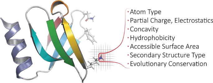
Calculated properties/features, biophysical and beyond. For each protein domain in Prop3D-20sf, we annotate every atom with the following features: atom type, element type, residue type, partial charge & electrostatics, concavity, hydrophobicity, accessible surface area, secondary structure type, and evolutionary conservation. For a full list of features used in Prop3D-20sf, see the text and Tables 3 and 4. In the ribbon diagram shown here (PDB1KQ2), a featurized (atomic) region is highlighted and demarcated in red, atop a voxelized background. Note that any bespoke feature can be defined and applied in Prop3D
Some of the properties mentioned above are computed at the residue level and mapped to each atom in the residue (e.g., hydrophobicity is one such property). That is, a ‘child’ atom inherits the value of a given feature from its ‘parent’ residue. For other features, residue-level values are calculated by combining atomic quantities, via various summation or averaging operations applied to the properties’ numerical values (as detailed in Table 3 for Prop3D-20sf). To illustrate the principle that residue-level properties may be directly/simply or indirectly/complexly related to atomic properties, consider that (i) the mass of a residue is a simple summation of the atomic masses of each of its constituent atoms, whereas (ii) properties such as residue volume or accessible surface area are not so straightforwardly derived from atomic properties, instead requiring the application of geometric methods (e.g., the Shrake-Rupley numerical algorithm [45]).
While all of the possible features are contained in the Prop3D-20sf dataset and undoubtedly will be somewhat correlated, it is possible for one to select only certain subsets of features of interest. We also create subsets of the Boolean features that we have found to be minimally correlated [46], and those can be selected, for example, in training deep neural networks.
As illustrative use-cases, we supply three nontrivial ML examples that involve representing proteins as sequences, graphs, or full 3D structures. At the sequence level, we present an example that uses Prop3D together with the language model–based Evolutionary Scale Model approach (ESM-2 [47]) to predict and annotate residue-level properties. Next, we illustrate how Prop3D can be used with ProteinMPNN [48], which is a recent deep learning approach for protein sequence design wherein structural information is encoded as graph neural networks, in order to predict residue-level features. And, finally, we briefly highlight a new DeepUrfold framework [12], where Prop3D is instrumental in creating superfamily-specific deep convolutional variational autoencoder (VAE) models at the level of full, intact 3D structures. These three sets of examples (complete with Python code), along with much other documentation, can be found at https://prop3d.readthedocs.io.
Dataset design and open data format (with some historical context)
In order to handle the large amount of protein data in massively parallel workflows, we engineered Prop3D to employ the Hierarchical Data Format (HDF5 [49]), along with the Highly Scalable Data Service (HSDS). We find the HDF5 file format to be a useful way to store and access immense protein datasets because it allows Prop3D to chunk/compress/navigate a protein structure hierarchy like CATH in a scalable and efficient manner. Using this approach versus, for example, creating myriad individual files spread across multiple directories, we can combine the data into ‘single’ files/objects that are easily shareable and can be accessed via a hierarchical structure of groups and datasets, each with attached metadata descriptors; note that hierarchical schemes, such as CATH, will generally lend themselves naturally to this sort of approach. Moreover, the HSDS extension to this object storage system allows multiple readers and writers which, in combination with Toil, affords a degree of parallelization that significantly accelerates the creation of new datasets, e.g. as part of a Prop3D-enabled workflow.
Many computational biologists have begun migrating to approaches such as HDF5 [50,51,52] and HSDS [53] in recent years because (i) binary data can be rapidly retrieved/read, (ii) such data are readily manipulable and easily shareable, and (iii) these systems provide well-integrated metadata and other beneficial services, schema and features (thus, e.g., facilitating attribution of data provenance). Before the relatively recent advent of HDF5(/HSDS) and other binary formats, biological data exchange and archival formats for protein 3D structures largely relied on human-readable, plaintext ASCII files (i.e., PDB files). For decades, PDB files have been the de facto standard format for sharing, storing and processing protein structure data, such as in structural bioinformatics workflows. Originally developed in 1976 to work with punch cards, the legacy PDB format is an ASCII file with fixed-column width and maximally 80 characters per line [54]. Working with traditional PDB files, a structure could be attributed with only one type of biophysical property, e.g., by substituting the numerical values of the desired property into the B-factor column—a highly limited workaround. Because of the inflexibility of the legacy PDB file and its limitations as a data exchange format, the macromolecular Crystallographic Information File (mmCIF) was developed; this file format was designed for better extensibility, flexibility and robustness (e.g., a standardized data dictionary), allowing for a 3D structure to be attributed with a plethora of properties, biophysical and otherwise [55]. Most recently, spurred by the slow nature of reading ASCII files, the Macromolecular Transmission Format (MMTF) has been developed to store protein structures in a compact binary format, based on MessagePack format (version 5) [56, 57]. While the MMTF is almost ideal for ML tasks, it still relies on using individual files in a file system, with no efficient, distributed mechanism to read in all files, no way to include metadata higher than residue level, and no ability to combine train/test splits directly into the schema—these were some of our motivating factors in adopting HDF5 and HSDS capabilities in Prop3D.
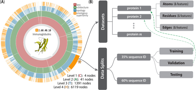
The CATH-inspired hierarchical structure of Prop3D. The inherently hierarchical structure of CATH (A) is echoed in the design schema underlying the Prop3D-20sf dataset (B), as illustrated here. Prop3D can be accessed as an HDF5 file seeded with the CATH hierarchy for all available superfamilies. For clarity, an example of one such superfamily is the individual H-group 2.60.40.10 (Immunoglobulins), shown here as the orange sector (denoted by an asterisk near 4 o’clock). Each such superfamily is further split into (i) the domain groups, with datasets provided for each domain (atomic features, residue features, and edge features), as delineated in the upper-half of (B), and (ii) pre-calculated data splits, shown in the lower-half of (B), which exist as hard-links (denoted as dashed green lines) to domain groups. (The ‘sunburst’ style CATH diagram, from http://cathdb.info, is under the Creative Commons Attribution 4.0 International License.)
For Prop3D and Prop3D-20sf, an HDF5 file is built by starting with the CATH database, which provides a hierarchical schema—namely, Class \(\supset\) Architecture \(\supset\) Topology \(\supset\) Homologous Superfamily—that is naturally amenable to parallelization and efficient data traversal, as shown in Fig. 6. In Prop3D, a superfamily can be accessed by its CATH code as the group key (e.g., ‘2/60/40/10’ for Immunoglobulin). We then split each superfamily into two groups (Fig. 6): (i) a ‘domains’ dataset, containing groups for each protein domain inside that superfamily (Fig. 6B, top half), and (ii) ‘data_splits’ (Fig. 6B, bottom half), containing pre-computed train (80%), validation (10%), and test (10%) data splits for use in developing ML models, where each domain in each split is hard-linked to the group for that domain (dashed green arrows in Fig. 6). Each domain group contains datasets for different types of features: ‘Atoms’, ‘Residues’ and ‘Edges’. The ‘Atoms’ dataset contains information drawn from the PDB file’s ATOM field, as well as all of the biophysical properties that we calculated for each atom. ‘Residues’ contains biophysical properties of each residue and position (average of all of its daughter atoms), e.g. for use in coarse-grained models. Finally, ‘Edges’ contains properties for each residue \(\leftrightarrow\) residue interaction, thereby enabling the construction and annotation of, e.g., contact maps in graph-based representations/models.
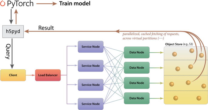
In terms of data-processing pipelines, HSDS allows HDF5 data stores to be hosted in S3-like buckets, such as AWS or MinIO, remotely and with accessibility achieved via a ReST API. HSDS data nodes and service nodes (Fig. 7) are controlled via a load-balancer in Kubernetes in order to enable efficient, distributed mechanisms to query HDF5 data stores, as well as write data with a quick, efficient, distributed mechanism; these properties of HSDS are achieved via various features of its engineering, including using data-caching and implicit parallelization of the task mapping across virtual partitions (Fig. 7). HSDS allows for multiple readers and multiple writers to read or write to the same file simultaneously, using a ‘distributed’ HDF5 multi-reader/multi-writer Python library known as h5pyd (Fig. 7). As part of Prop3D, we have setup a local k3s instance, which is an easy-to-install, lightweight distribution of Kubernetes that can run on a single machine along with MinIO S3 buckets. We have found this approach to be particularly useful in enabling flexible scalability: our solution works on HPC data infrastructures that can be either large or (relatively) small.
Cloud-based access to the Prop3D-20sf Dataset via HSDS. HSDS creates Service Nodes, which are containers that handle query requests from clients, and Data Nodes, which are containers that access the object storage in an efficient, distributed manner. The Prop3D-20sf dataset can be used as input to train an ML model either by accessing the data via a Python client library (h5pyd) or through our separate DeepUrfold Python package, which supplies PyTorch data loaders [12]. This illustration was adapted from one that can be found at the HSDS webpage (available under an Apache 2.0 license, which is compatible with CC-by\(-\)4.0)
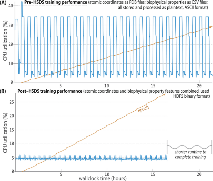
In creating the Prop3D-20sf dataset, HSDS, in combination with a Toil-enabled workflow, allows for each parallelized task to write to the same HDF5 data store simultaneously. The Prop3D-20sf dataset can be read in parallel as well, e.g. in PyTorch. We provide PyTorch Data Loaders to read the Prop3D-20sf dataset from an HSDS endpoint using multiple processes; that functionality is available in our related DeepUrfold Python package [12]. Promisingly, we found that when HSDS was used with Prop3D as a system for distributed training of deep generative models in our DeepUrfold ML workflow, as opposed to using raw ASCII files, a speedup of \(\approx \,\)33% (8 h) was achieved, corresponding to a reduction from \(\approx \,\)24 h to \(\approx \,\)16 h of wall-clock time to train an immunoglobulin-specific variational autoencoder model with 25,524 featurized Ig domain structures (Fig. 8). Thus, we found it clearly and significantly advantageous to utilize the parallelizable data-handler capacity that is provided by a remote, cloud-based, parallel-processing system like HSDS.
HSDS affords significantly improved training runtimes. Using Prop3D, we trained an immunoglobulin-specific variational autoencoder with \(\approx \,\)25K domain structures, employing 64 CPUs to process data and four GPUs for 30 epochs of training (orange trace; [12]). A Before we chose to implement HSDS in Prop3D, we stored and processed domain structures as simple plaintext PDB files (parsed with BioPython), along with the corresponding biophysical properties for all atoms in these structures as plaintext files of comma-separated values (CSV; parsed with Pandas). That computation took \(\approx \,\)24 h of wallclock time for \(\approx \,\)50K ASCII files on a well-equipped GPU workstation. B. Reformulating and streamlining the Prop3D pipeline with HSDS yielded a substantial (\(\approx \,\)33%) speed-up: training runtimes across many epochs (orange) improved by \(\approx \,\)8 h (to \(\approx \,\)16 h total), with there being far more efficient CPU usage while reading all of the data (blue traces; note the different vertical scales in A and B). These data-panel images were exported from our Weights and Biases training dashboard

