Study setting
This study was performed at the University Medical Center Groningen (UMCG), a 1339-bed academic tertiary care hospital in the North of the Netherlands. Ethical approval was obtained from the institutional review board (Medical Ethical Committee) of the UMCG, and informed consent was waived by this committee due to the retrospective observational nature of the study (METc 2018/081). The study was performed in accordance with relevant local, national and international guidelines/regulations. It included patients admitted to the 42-bed multidisciplinary adult critical care department with several ICUs at the UMCG. All patients were admitted between March 3, 2014, and December 2, 2017, based on the use and database availability of the local EHR system during this time. Patients were included in this study if they were registered in this EHR system, did not object to their use of data in the UMCG objection registry, and were at least 18 years old at the time of ICU admission. All patient data was anonymised prior to analysis.
Infection-related consultations
Consultations analysed in this study were performed by clinical microbiologists and ID specialists of the hospital’s Department of Medical Microbiology and Infection Prevention. This department is responsible for all microbiological and infection control/prevention services at the UMCG. It offers a full spectrum of state-of-the-art diagnostic procedures for rapid, precise, and patient-specific diagnosis of infections. The department provides consulting assistance to the ICU in the form of a dedicated clinical microbiologist/ID specialist with 24/7 availability. Consultations at the ICU were triggered through various ways: (1) clinically-triggered by request from intensivists, (2) laboratory-triggered by pertinent diagnostic findings, (3) routine monitoring of newly admitted patients by a clinical microbiologist/ID specialist, or (4) by regular in-person participation in clinical rounds at the ICU which can also result in proactive “by-catch” consultations. In addition, the clinical microbiologist/ID specialist in charge attends the daily ICU multidisciplinary patient board. All consultations were recorded in the local database at the Department of Medical Microbiology and Infection Prevention.
Data extraction and processing
Data was extracted from local EHR systems. The ICU EHR system comprised 1909 raw features (variables) covering all laboratory results, point-of-care test results, vital signs, line placements, and prescriptions. Demographic and administrative patient information was extracted from an administrative hospital database. Infection-related consultation timestamps per patient were obtained from the laboratory information system (LIS) at the Department of Medical Microbiology and Infection Control. All data were cleaned to remove duplicates, extract numeric values coded in text, and standardize time stamps where appropriate.
Laboratory and point-of-care test results were included if at least one data point per feature was available in at least 30% of all patient admissions. This resulted in 121 features. Numeric features were cleaned to exclude outliers (physiologically impossible values), which typically indicated faulty tests or missing test specimens. All feature timestamps were available at the minute level. For numeric features the mean per minute was taken if more than one data point per minute was available. No double entries per minute were observed for categorical values. Categorical values indicating missing specimens or other error messages (e.g., “wrong material sent”) were transformed to missing values. Laboratory features were re-coded to indicate if values fell in between feature-specific reference ranges based on available, local reference values.
Raw vital signs were cleaned for outliers (e.g., systolic arterial blood pressure smaller than diastolic arterial blood pressure), which usually indicated faulty measurements (e.g., through kinked lines). Line placement data was transformed to a binary feature indicating the presence or absence of an intravenous or arterial line per minute and line type. Prescription data were filtered to include prescriptions of the categories: antimicrobials (identified through agent specific codes in the EHR), blood products, circulatory/diuresis, colloids, crystalloids, haemostasis, inhalation, cardiopulmonary resuscitation, and sedatives. All prescriptions were transformed to binary features indicating the presence of a prescription per minute, agent, and type of administration. Additional binary features were introduced indicating the presence of a prescription per prescription category and type of administration. Dosing was available but not in standardized format and therefore omitted. Selective digestive decontamination (SDD) is a standard procedure in our hospital and was thus indicated by a distinct variable to avoid confusion with antimicrobial agents for other purposes20.
To prevent sparseness, all time dependent data were aggregated per 8-h intervals (arbitrary virtual shifts) of the respective ICU stay. We chose to aggregate the data to arbitrary virtual 8-h shifts to mimic clinicians’ behaviour in reviewing what took place the previous shift before making medical decisions in the current shift. The aggregation was done by taking the mean value over the 8-h interval or taking the occurrence of an event in the case of dichotomized features. For laboratory values, the last observation was used, which we have operationally defined as clinically the most relevant observation. Supplementary Table 1 shows an overview of the missing data after 8-h aggregation. Of note, missing data for laboratory and point of care tests, prescriptions and line placements are either truly missing, or missing because the action was not performed. However, due to the importance of having correct data for these features for clinical reasoning, we assumed that these features were missing for the latter reason. Missing values were filled with the last available data point before the missing value21. This carry-forward imputation process was used to mimic common physician’s behaviour. Remaining missing numeric values were imputed using the median of the feature’s overall distribution. Near zero variance predictors (features not showing a significant variance) were dropped from the dataset at a ratio of 95/5 for the most common to the second most common value. Each patient’s stay was treated as an independent stay, but a readmission feature was introduced, indicating how often the patient was previously admitted during the study period.
Consultation data included the time of documentation of infection-related consultations for patients admitted to the ICU. These include a variable delay between action and documentation, and a non-standardized free text documentation. The type of consultation (i.e., via phone or in person) was not available. Data were filtered to identify the first consultation time stamp per patient and admission. This point in time formed the targeted outcome of this study. Subsequent consultations were disregarded as they involve follow up on the clinical course of the initially presented problem and are therefore largely clinically predictable. Moreover, predictions of later consultations will consequently lead to only nominal time gain. The final dataset used in the modelling process comprised 104 features (see Supplementary Table 2). An overview of the study design including the data processing is shown in Fig. 1.
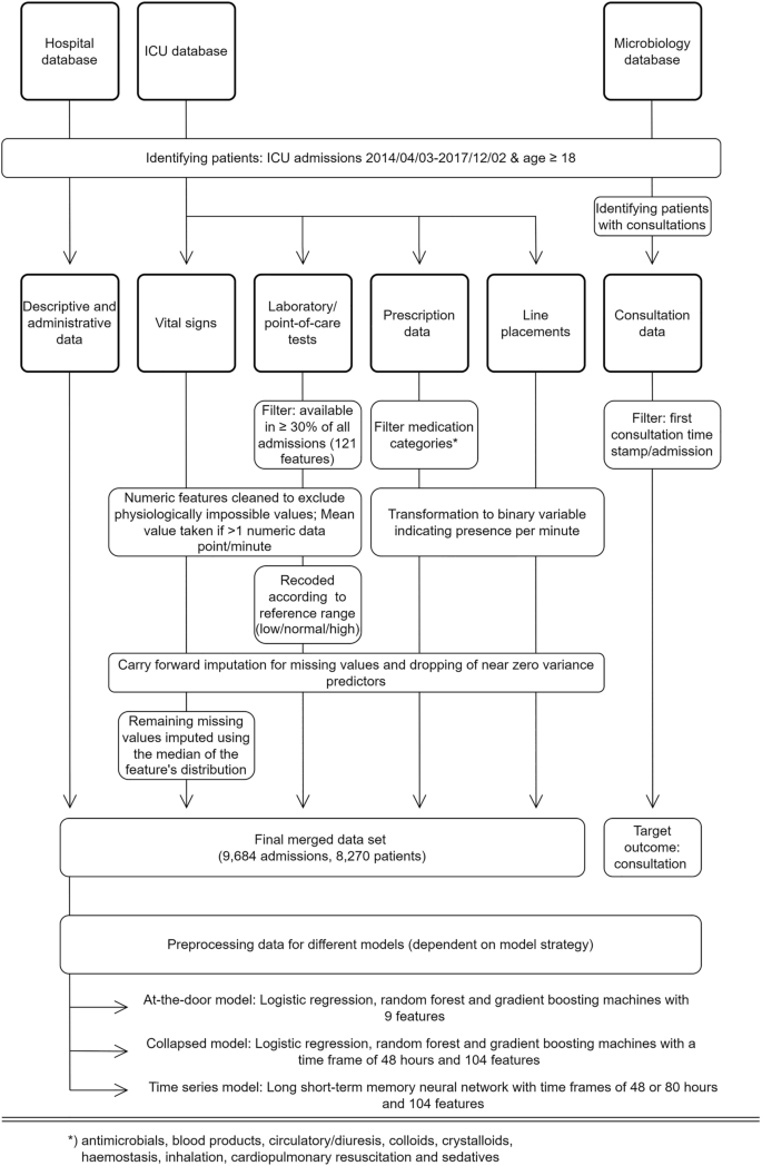
Study design and data processing for three different data sources (hospital database, ICU database, and medical microbiology database). Note: (interim) microbiology reports were not included in the modelling process. Standard data cleaning processes are not shown (cf. main text in “Methods”).
Cohort investigation
Descriptive analyses were stratified by consultation status (consultation vs. no consultation). Baseline patient characteristics were assessed and compared with Fisher’s exact test for categorical features and Student’s t-test for continuous features. Logistic regression was used to create an explanatory model for infection-related consultations using the baseline features. Odds ratios with 95% confidence interval were used in the result presentation.
Modelling process
Three different modelling approaches were used and evaluated in this study to predict an infection-related consultation. Each model made one prediction per patient and admission (i.e., sequence-to-one classification). The first approach (at-the-door model) used static patient features available at the time of admission: gender, age, body mass index, weekend admission, mechanical ventilation at admission, referring specialty, planned admission, readmission, and admission via the operation room. We used two outstanding powerful ensemble models, random forest (RF)22, and gradient boosting machines (GBM)23, and a commonly used generalised linear model (i.e. logistic regression)24 to predict the need for an infection-related consultation at any time during a patient’s stay in the ICU. Predictions were made at the time of the admission to the ICU.
The second modelling approach (collapsed model) also used LR, RF, and GBM and additional time-dependent procedural features measured during the ICU stay, such as the presence of medication, lines, performed diagnostics, and vital signs (see Supplementary Table 2) to predict a consultation up to eight hours (one arbitrary virtual shift) in advance. Since LR, RF, and GBM are not suited to handle raw longitudinal data, an additional pre-processing step was required. To enable the inclusion of time dependent features in the model, longitudinal data were aggregated to predict the target event (infection-related consultation) by calculating the mean, the standard deviation, minimum, maximum and trend over the available data. In the case of dichotomised variables, time series were aggregated by taking the proportions over time. Aggregation was done over a time span of 48 h. In case that patients stayed less than 48 h on the ICU all available data were aggregated. The arbitrary virtual shift in which the consultation took place was not included in the aggregation. The aggregation process led to missing values for the standard deviations and trends in the case that patients had less than two observations prior to a consultation. The RF and GBM models, as a standard feature, are able to handle these missing values. For the LR all observations with missing values were removed prior to the analysis (3405 admissions). This led to a dataset with 6279 admissions for the LR. For completeness the RF and GBM models were trained and evaluated on a dataset with and without missing values.
The aggregated data were used to predict the need for a consultation in the next arbitrary virtual shift (i.e., between zero and eight hours in advance). For patients receiving a consultation the 48 h of aggregated data before the shift in which the consultation took place were used to predict a consultation in the next arbitrary virtual shift. To create an unbiased ending point for patients who did not receive a consultation we used 48 h of aggregated data up to a random point during their ICU stay to predict the event (i.e., infection-related consultation or not) in the next arbitrary virtual shift. This ending point was randomly taken between one arbitrary virtual shift after admission up to one arbitrary virtual shift before discharge.
The third approach used a long short-term memory neural network (LSTM) to model the target outcome (time-series model). LSTM is an artificial recurrent neural network with the advantage to include memory and feedback into the model architecture. This time-aware nature (and its similarity to clinical reasoning) in addition to previous reports on the beneficial use of LSTM in the field of infection management with EHR built the background for the choice of this methodology25,26,27. An LSTM has the advantage that the data did not need to be aggregated to be used in the model, but all available information could be used without the need for additional feature pre-processing. Following the same approach as for the collapsed model, the LSTM model included all available features (see Supplementary Table 2). To prepare the model for the LSTM, data were split into arbitrary virtual 8-h shifts of a given ICU stay. Each of these arbitrary virtual shifts represented one time step in the model. Two different LSTM models were trained. First and similar to the collapsed approach, a time frame of 48 h (i.e., six virtual arbitrary shifts) was used to predict the occurrence of an infection-related consultation in the next virtual arbitrary shift. Finally, a second LSTM model used a time frame of 80 h (i.e., ten virtual arbitrary shifts) to predict infection-related consultations in the next virtual arbitrary shift. The virtual arbitrary shift in which the consultation took place was not included in the data used to make the prediction. The different shifts (i.e., six or ten virtual arbitrary shifts) of the data were used to predict an infection-related consultation in the seventh or eleventh virtual arbitrary shift, respectively. To create an unbiased endpoint for patients who did not receive a consultation we used the different shifts (i.e., six or ten virtual arbitrary shifts) of the data up to a random point during their ICU stay to predict the event (i.e., infection-related consultation or not) in the next virtual arbitrary shift. This random point was taken between one virtual arbitrary shift after admission up to one arbitrary virtual shift before discharge. Data for patients who had length of stay shorter than six or ten arbitrary virtual shifts were padded to ensure inputs of the same size.
The time-series models were trained with and without the use of standard deviations of each time dependent feature within each arbitrary virtual shift. Laboratory values were an exception to this as most laboratory results were less frequent than once per arbitrary virtual shifts. In that case, the standard deviation is undefined leading to many missing values. Therefore, no standard deviations were taken for laboratory values.
Training, optimization, and evaluation of the models
The data was randomly split into a train and a test set using an 80-20 split. All models were trained and evaluated on the same train and held-out test set. Fisher’s exact test for categorical features and Student’s t-test for continuous features were performed for the target and all baseline characteristics on the train and held-out test set to ensure similar baseline characteristics. Model performances were evaluated and compared using the area under the receiver operating curve (AUROC) and the area under the precision recall curve (AUPRC).
All machine learning models were trained with and without addressing class imbalance. For the at-the-door and collapsed models class imbalance was addressed using oversampling. For the time-series models class imbalance was addressed using higher class weights for the minority class. All models were evaluated using tenfold cross validation. Confidence intervals of the performance on the validation set were calculated using the results on the different validation folds. A random grid search was used to select the optimal hyperparameters for the at-the-door models as well as the collapsed models. For the RF we used a thousand trees and for the GBM we used 5000 trees. However, we tested if 2000 or 6000 trees increased performance. An early stopping was applied to both models, where the moving average of the ten best stopping rounds was compared to the most recent stopping round and if performance did not increase substantially no trees were added (i.e., stopping_rounds = 10). For both the RF as well as the GBM a grid search was performed on the minimum number of observations in a leaf to split (min_rows), the maximum tree depth (max_depth) and the number of observations per tree (sample_rate). For RF we additionally searched for the optimal value for the number of features to sample at each split (mtry). Moreover, for the GBM a grid search was performed on the number of features per tree (col_sample_rate), the learning rate (learn_rate) and the reduction in the learning rate after every tree (learn_rate_annealing). The LSTM model was manually tuned on the validation folds by adding layers, adjusting the number of units, the drop out and batch size. The effects of these model adjustments were monitored using learning curves per epoch displaying the train and validation performance. Calibration plots, calibration intercepts and slopes, scaled Brier score, decision curve analysis, and feature importance plots were analysed for all best performing models per modelling approach. Finally, we analysed the model performance of all best performing models per modelling approach on sub-populations with different characteristics (e.g. planned admissions, post-operative patients).
All data processing and analyses were performed using tidyverse and H2O in R and numpy, pandas, caret, scikit-learn, keras, and tensorflow in Python28,29. The data is registered in the Groningen Data Catalogue (https://groningendatacatalogus.nl). The study followed the Transparent Reporting of a Multivariable Prediction Model for Individual Prognosis or Diagnosis (TRIPOD) statement (template available in Supplementary Table 3)30.