Evaluating the pedestrian level of service for varying trip purposes using machine learning algorithms

The models are developed using Random Forest and Light GBM algorithms which also include testing for prediction accuracy. The choice of the 80–20 percent split in the use of data corresponds to the training set and the test set respectively as explained before. The metrics such as accuracy, precision, recall, and f-score are used to evaluate the performance of models which is shown in Table 3. Due to a smaller number of pedestrians rating the LOS of roads as 1 or very poor, the data corresponding to ratings 1 and 2 has been combined as ‘1’. Hence the five levels of service are reduced to four and the percentage of data collected for each class and trip purpose is shown in Table 1. While explaining the feature analysis and working of the model, class 3 represents PLOS A, class 2 represents PLOS B, class 1 stands for PLOS C, and finally class 0 stands for PLOS D.

Table 3 Metrics of the machine learning models.

From Table 3 it is observed that the Light GBM model performs more accurately than the Random Forest model for Education and Recreation trip purposes. It works out to be 10% and 5% more accurate than the Random Forest model by giving accuracy scores of 0.74 and 0.80 and f1-scores of 0.71 and 0.81. The sensitivity of the models seems to be slightly higher for Education and Recreation trip purposes when evaluated using Light GBM models. The accuracy, sensitivity, and f1- scores of the models for Work trip purposes are almost the same for both the machine learning models. To further estimate the predictive capability of the two machine learning models the AUROC (Area under the receiver operating characteristic curve) value can be used⁴¹. The area under the curve gives an idea of how well a model can help to identify the classes of a response variable. In multiclass classification, the AUC curve is determined by binarizing the output as one vs rest or one vs one. In this case, one vs rest is used to find the value of AUROC which is shown in Table 4. It shows that the AUROC values are slightly higher for the Light GBM models for all three trip purposes. Hence the light GBM model will be analysed further using a model agnostic method based on game theory, called SHAP to understand its features and the results.

Table 4 ROC-AUC values for the different models.

Feature importance using SHAP

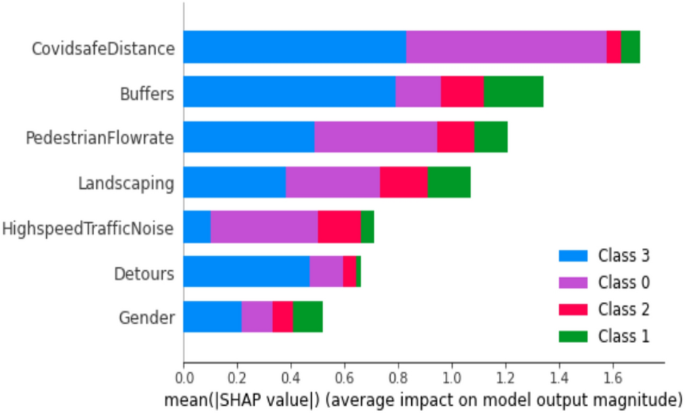
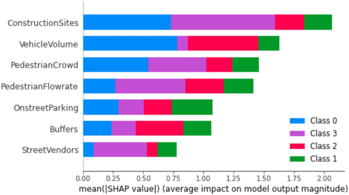
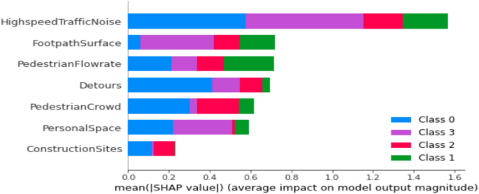
The SHAP summary plot serves as a tool to elucidate the features that hold greater significance in predicting the pedestrian level of service (PLOS) within the model. Additionally, it aids in identifying features that specifically influence a particular class, offering a comprehensive, global interpretation of the model. On this plot, the Y-axis denotes the feature names arranged in descending order of importance, reflecting their impact on the model’s output. Meanwhile, the X-axis represents the mean absolute Shapley values, providing a measure of the magnitude of feature attributions. This graphical representation offers a clear visualization of the relative importance of features in shaping the predictions and understanding the model’s overall behaviour.

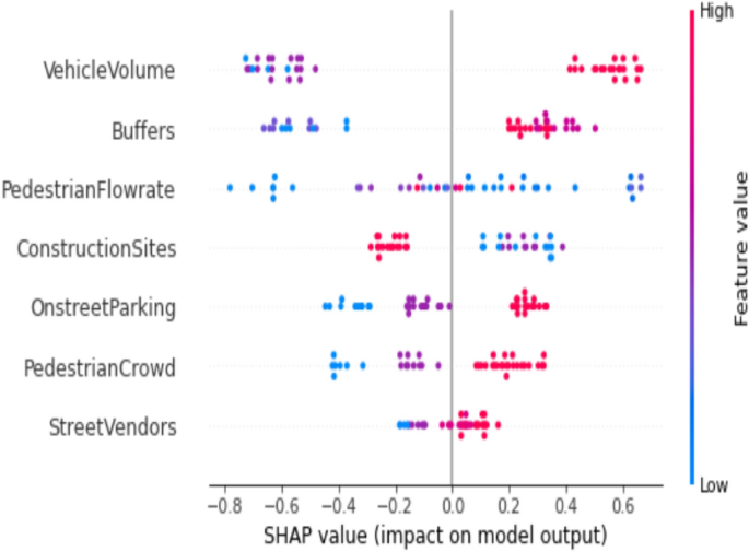
Lundberg and Lee^42,43 discovered that commonly employed methods such as feature importance permutation and a mean decrease in impurity fail to meet the criteria of consistency and accuracy. These criteria entail that the cumulative contributions of each feature should equate to the total contribution in the model. The feature importance of models for three trip purposes is depicted in Figs. 5, 6, and 7. Notably, the pivotal features for educational trips, as indicated in Fig. 5, encompass interpersonal space between pedestrians, safe distance from vehicles on the road, and pedestrian speed. These factors significantly contribute to predicting the four categories of PLOS. Conversely, for recreational trips, Fig. 6 reveals that PLOS is chiefly influenced by construction sites, vehicle volume, and pedestrian crowd. Numerous locations in the central city witness detours caused by construction zones, particularly during pedestrian walks.

Figure 7 illustrates that individuals walking in the city for work-related purposes prioritize certain factors in the prediction of PLOS. These factors include traffic noise, footpath surface, detours, and pedestrian speed. Notably, construction sites only impact PLOS A and B without affecting other levels of service. This model provides valuable insights into the behaviour of pedestrians traversing city walkways, effectively capturing preferences based on different destinations.

The model effectively reveals distinct preferences among pedestrians. For instance, students walking to universities focus primarily on maintaining a suitable distance from others and vehicles, along with the ability to walk at a pace conducive to reaching their classes on time. Pedestrian density and vehicle volume are of lesser concern to them. It’s worth noting that educational sites, where the data was collected, experience a significant surge in pedestrian volume during daytime class hours. On the other hand, pedestrians strolling for recreational purposes express discomfort with high pedestrian density, substantial vehicle volume, and interruptions caused by construction activities on footpaths. These factors hinder the enjoyment of their walk on the footpaths. For commuters heading to work, footpath usage is routine, and they are acutely aware of pedestrian density and vehicle volume during their typical travel times. Their concerns include traffic noise on busy roads, a desire for a clean footpath surface free of spilled food or trip hazards, and apprehension about unexpected detours that might extend travel time and alter walking speed on footpaths.

SHAP summary plot

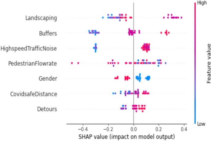
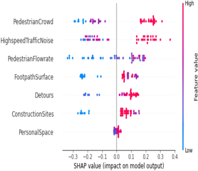
The influence of a feature on the class is aggregated to create a plot illustrating the feature’s importance for that class. In this summary plot, each point corresponds to a Shapely value of the feature at a specific instance. The y-axis signifies the ranking of feature importance for the model’s output, while the x-axis is determined by the SHAP value, representing the magnitude of change in log odds. In this graphical representation, points are denoted in both blue and red, where blue signifies a low value of the feature, while red indicates a high value of the feature. This colour coding effectively highlights the impact of feature values on the model’s output, providing a visual representation of their relative importance.

Figure 8 highlights the impact of landscaping and minimal disturbance of traffic noise on the pedestrian level of service (PLOS) for footpaths in educational areas. Points marked in red emphasize that higher ratings for landscape and minimal traffic noise directly contribute to an elevated PLOS, indicating a higher level of comfort. Specifically, in instances where a good level of service is observed, pedestrians on the footpath prioritize factors such as maintaining a safe distance from vehicles on the road, minimizing traffic noise, and enjoying a walkway adorned with trees and a refreshing landscape. These considerations underscore the importance of environmental elements in influencing the perceived comfort and quality of footpaths in educational settings.

Figure 9 represents the model output for Pedestrian Level of Service (PLOS) in recreational areas, specifically focusing on a good level of comfort corresponding to PLOS B. In instances where a better PLOS is observed, pedestrians express a preference for specific conditions. Pedestrians, aiming for a good PLOS in recreational areas, show a preference for lower vehicle volumes on the adjacent roads. They also desire a safe distance from vehicles traveling on the road. Additionally, a key factor contributing to a favourable PLOS is the absence of disruptions on the footpath caused by construction activities. These insights underscore the importance of factors such as reduced traffic, safety from vehicles, and uninterrupted footpaths in enhancing the perceived comfort of pedestrians in recreational areas.

The inference drawn from Fig. 10, particularly for instances reflecting a good comfort level, indicates that red points, denoting higher comfort ratings, have a positive impact on the Pedestrian Level of Service (PLOS) rating for PLOS B. Specifically, the factors contributing to this positive impact include experiencing lower pedestrian density around them, reduced traffic noise on the road, and the ability to walk at the required speed on footpaths.

The utilization of the SHAP technique across all three trip purposes in deriving this explanation underscores the reliability of the Light GBM model in predicting the Level of Service (LOS). The consistency of these findings across various trip purposes highlights the robustness and generalizability of the model’s predictions, reinforcing its trustworthiness in assessing and predicting pedestrian experiences across different scenarios.

Waterfall plot

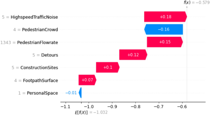
So far, SHAP has been used to determine the impact of individual features on model predictions for global interpretation. Additionally, it has been applied to a specific class of LOS for footpaths. SHAP also explains how features affect a single instance of prediction, providing local interpretation. It helps to explain, for a specific class and at a specific row of Shapley values, which variables improve the PLOS and which features reduce the rating of PLOS. SHAP waterfall plots assist in identifying how the model arrived at a prediction for a single observation.

In Fig. 11, we observe that f(x) represents the model-predicted probability value for LOS (level of service) B, while E[f(x)] is the base value. The values of the features to the left correspond to the actual observations in the data, and the values on the arrows represent the Shapley values of the features. The red arrows indicate a positive effect of the features, increasing the base value, while the blue arrows indicate a negative effect, aiming to reduce the base value to ultimately yield the predicted model value. In this case, we observe that features such as discomfort experienced by the surrounding crowd and the inability to maintain personal space are negatively impacting the PLOS, leading to a reduction in its rating.