Diffusion-based generative AI for exploring transition states from 2D molecular graphs

A brief description of the generation process

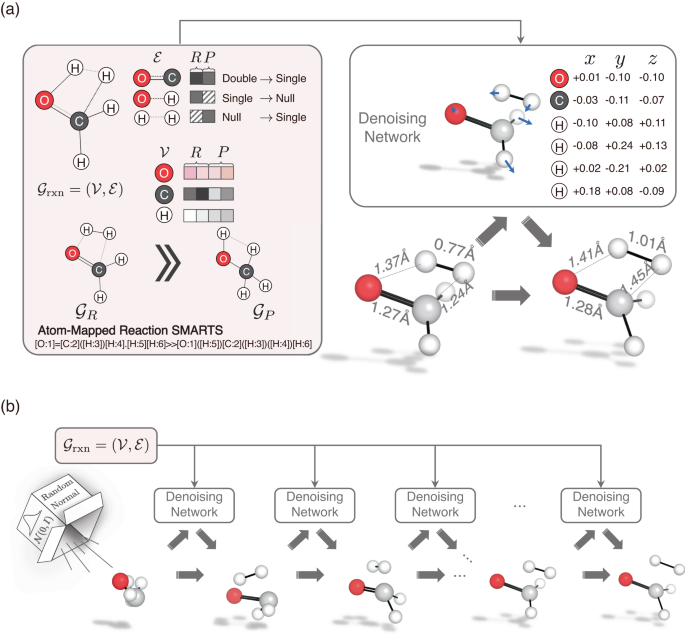
In this section, we provide a brief overview of TSDiff, an ML model designed to learn the conditional distribution of 3D TS geometries given 2D reaction information presented as SMARTS⁵⁵ (see Fig. 1a). TSDiff is based on the stochastic denoising diffusion method, where the model is trained to learn the reverse process of a noise process that adds a random noise to the given geometry at each discrete time step. At the inference phase, TS geometries are generated from an initial state with a complete noise through the iterative denoising process, where the noisy input is gradually refined by the denoising neural network at each time step, given the 2D reaction information (see Fig. 1b).

**Fig. 1: Overview of the proposed TSDiff.**

The input of the model is 2D reaction information expressed as a reaction graph \({{{{{{{{\mathcal{G}}}}}}}}}_{{{{{{{{\rm{rxn}}}}}}}}}\) which captures the bond changes in reactants and products⁵⁶. The simplified version of the reaction graph is depicted in the left box of Fig. 1a. Molecular graphs for reactants and products, \({{{{{{{{\mathcal{G}}}}}}}}}_{R}\) and \({{{{{{{{\mathcal{G}}}}}}}}}_{P}\), can be constructed based on bond and atom information that can be obtained from SMILES⁵⁷. The nodes in the graph are represented as atom-feature vectors containing atomic numbers. For the edges, the molecular graphs utilize extended graph edges that include node-pair indices within a 3-hop graph distance in the raw graph created based on covalent bonds. The condensed reaction graph, which serves as our model input, is formed by combining the two graphs of reactants and products using atom-mapping information.

TSDiff employs graph neural network (GNN) layers based on SchNet⁵⁸ for its denoising neural network to handle the noisy positions and reaction graphs. The construction of a geometric reaction graph involves adding the noisy positions to the 2D reaction graph and connecting nodes with interatomic distances smaller than a specified cutoff radius. This process integrates bond information, graph distance information, and spatial distance information as edge-features in the geometric graph. Subsequently, the model leverages these geometric reaction graphs to approximate a score function, a gradient of log-likelihood for noisy TS conformations, which is applied to denoising by updating the noisy positions toward the correct TS geometry. More details are described in the TSDiff section.

The proposed TSDiff was trained and validated using the general organic gas-phase reaction database published by Grambow et al.⁴³. We employed an ensemble with a total of eight models, and our training process took 22 h for each model on a single RTX 2080 Ti NVIDIA GPU. For most results reported in the following sections, we used the ensemble model and will refer to it as TSDiff unless otherwise noted. Diffusion models entail higher inference costs compared to other deep learning models, mainly due to their iterative denoising process. Specifically, TSDiff requires 5000 denoising steps for inference, which takes a few seconds per reaction. However, this cost is negligible compared to DFT calculations for TS optimization.

Generation of TS conformations

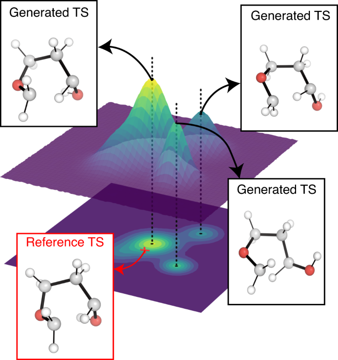
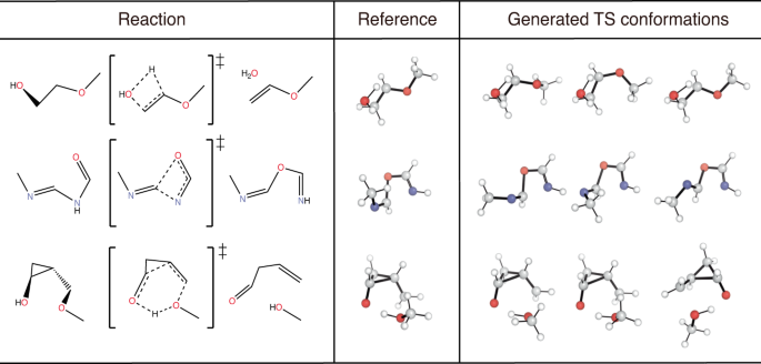
We emphasize that TSDiff is a stochastic generative model, implying that different geometries are generated at each sampling. Figure 2 depicts a conceptual representation of TSDiff’s predictive distribution. The different geometries generated by TSDiff correspond to specific TS conformations that can be built from the same 2D reaction graph. For example, Fig. 3 shows several generated geometries corresponding to specific conformations and reference geometries for three reactions in the test set. This is an inherent outcome because TSDiff uses only 2D graphs as input. Also, the reference TS would be one of various TS conformations identified by a specific computational method. Therefore, it is essential to consider diverse conformations and the comparative analysis of their barrier heights in the TS exploration process in order to identify the most favorable reaction pathway. Thanks to the nature of generative AI, TSDiff learns the distribution of TS geometries for diverse reactions in training, facilitating the reliable sampling of these different TS conformations.

**Fig. 2: Conceptual illustration of predictive distribution of TSDiff.**

**Fig. 3: Examples of transition state (TS) conformations generated by TSDiff.**

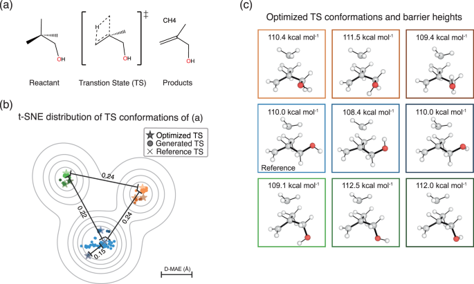
The various conformations generated by TSDiff need to be verified to ensure that they are indeed chemically valid TSs. As an example, we performed quantum chemical validation on a single test reaction. First, TSDiff generated one hundred samples for this reaction, which were then optimized using a saddle point optimization. Figure 4 visualizes the distribution of the generated geometries using t-distributed stochastic neighbor embedding (t-SNE)⁵⁹ in scikit-learn⁶⁰. Each dot in the figure represents a generated geometry, while the star and cross-shaped dots indicate the optimized and reference geometries, respectively. In addition, each dot has been color-coded to reflect its respective optimization result. For example, all generated geometries represented by the blue dots were optimized to the geometry represented by the blue star-shaped dot via the saddle point optimization.

**Fig. 4: Visualization of the geometries generated by TSDiff.**

All one hundred generated geometries were successfully optimized to saddle points, resulting in nine different TS conformations. The images on the right side of Fig. 4 show the optimized conformations. On the t-SNE projection map, it is evident that similar conformations tend to cluster together and be closely located to their respective optimized results. This character of the generated samples suggests that an efficient search for TS conformations is possible without having to perform quantum chemical calculations on the entire generated samples. Many clustering algorithms are already available, offering an effective means to select representative conformation samples. We also present an illustrative experiment in the Supplementary Discussion, showcasing the practical application of a clustering algorithm in TS exploration using TSDiff.

The nine different conformations were caused by two rotatable single bonds closest to oxygen, C–C and C–O. There were three major conformational changes with different dihedral angles centered on the C–C bond, and for each there were three minor conformations with different dihedral angles centered on the C–O bond, resulting in a total of nine different conformations. Here, the accuracy of the generated geometries was measured by the mean absolute error (MAE) of interatomic distances, D–MAE, with respect to their corresponding optimized results. A detailed method for measuring the D–MAE is given in the Measurement details section. The resulting average D–MAE was very small at 0.045 Å, indicating that the generated samples were optimized to the respective saddle points with only minor adjustments.

The resulting optimized geometries were all confirmed as valid TS geometries using IRC calculations. A detailed description of the IRC and validation method is provided in the Computational details section. This result indicates that TSDiff can find not only a conformation that corresponds to the reference geometry but also other valid TS conformations. Interestingly, the discovered TS conformations include TSs with lower barrier heights than that of the reference, as shown in Fig. 4, where the barrier heights were calculated with the energy difference between the optimized TSs and the reference reactants. This proves that the reference TS may not be the most favorable one, even though it was built using the most stable molecular conformation of the reactants⁴³, highlighting the importance of exploring multiple TS conformations. As a result, we demonstrate that the stochastic diffusion model, which has already shown its capability of accurately generating conformers in equilibrium, can be extended to TS explorations.

Performance of TS generation

From the perspective of a generative AI, it is important to evaluate the ability of TSDiff to generate samples that cover the reference TS of the dataset and how accurate the generated samples are. To this end, we calculated the following two metrics for all reactions in the test set: coverage (COV) and matching (MAT) scores. The COV score measures the percentage of reference TS geometries covered by the predicted ones by TSDiff, where a reference is considered to be covered if there exists any predicted one having a D–MAE within a criterion of δ with the reference. We used two criterion values: δ = 0.1 Å and δ = 0.2 Å. The value of 0.1 Å was determined based on the accuracy of a state-of-the-art model⁴⁰ that has demonstrated reliability with a high success rate in quantum chemical validations. However, this can be a strict criterion, so we also evaluated a COV score of δ = 0.2 Å. The MAT score measures the similarity between generated and reference samples by calculating the minimum D–MAE between the generated geometries and the reference geometry. The mathematical definitions of these two metrics can be found in the Measurement details section.

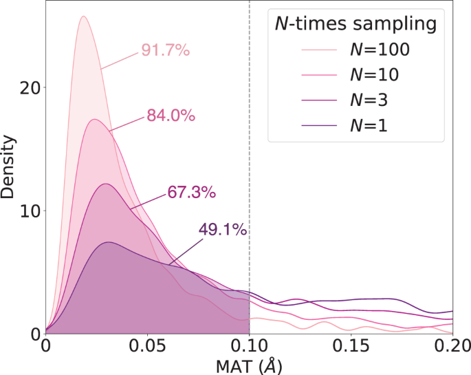
While these two metrics are widely used for generative AI evaluation, it should be noted that they have a limited application in this study because there is only one TS conformation for each reaction in the reference dataset. Therefore, for each individual reaction, the COV score is either 100% or 0% if only a single sample is used for evaluation. Thus, Table 1 presents the COV and MAT scores of TSDiff according to the number of sampling, including a comparison to the scores of TSDiff without the ensemble method. The distributions of the MAT scores across the reaction are shown in Fig. 5.

Table 1 The coverage (COV) and matching (MAT) scores of TSDiff according to the number of sampling

**Fig. 5: The distribution of the matching (MAT) scores of TSDiff with the number of sampling.**

The COV and MAT scores improve rapidly as the number of sampling increases. This is because TSDiff’s performance is underestimated at small numbers of the sampling, as it generates many different conformations, as shown in Fig. 3. In addition, the ensemble method led to slight performance improvements in both COV and MAT scores. As a result, TSDiff is expected to be able to generate 84.0% of the reference TSs with a D–MAE of 0.1 Å or less within ten rounds of sampling.

We compare the features and accuracies of TSDiff and the existing ML models in Table 2. To the best of our knowledge, Table 2 includes all the models whose performance has been reported on the Grambow’s dataset⁴³. Previous works commonly used geometries of reactants and products for their input features^37,38,39,40, and the most recently reported model by Choi additionally used the interpolated geometries of reactants and products⁴⁰. Their prediction targets are broadly divided into two categories: interatomic distances and atomic positions. The models that predict interatomic distances require an additional step of a nonlinear least-squares optimization to restore the distances to atomic positions. In contrast, Jackson et al. directly predicted atomic positions using tensor field networks³⁷. TSDiff also targets atomic positions directly in its generation process. A unique feature that distinguishes it from the existing models is that TSDiff uses only 2D graphs as input.

Table 2 Comparison of accuracy and features between machine learning models

Before comparing the accuracy of the models, it is important to note that evaluating the accuracy of TSDiff under the same conditions as existing models is not straightforward because TSDiff can generate other TS conformations, while we only have a single TS conformation available as a reference. To address this, we evaluated the accuracy of TSDiff on a TS conformation only if it directly matches the corresponding reference. To identify these matching samples, we conducted saddle point optimizations on the generated samples. For a reliable comparison, we aimed to find as many test reactions with a matched reference as possible, so we performed the optimization on TS conformations generated with a total of eight rounds of sampling for each reaction. Samples with a D–MAE between their optimized result and the reference of less than 0.01 Å were considered matching, resulting in the covering rates of 53.2% and 84.6% of the test reactions with one and eight sampling rounds, respectively. One of the generated samples is randomly selected to calculate the D–MAE when multiple samples match the same reference TS in a given reaction graph, which gives a consistent D–MAE value regardless of the number of sampling rounds to facilitate fair evaluation.

Table 2 shows the D–MAE values of TSDiff with and without considering conformer matching. The latter is the case for a single sampling, the resulting conformation of which can be considered an approximate TS for the respective reference. In this case, the D–MAE value is 0.137 Å, which is lower than those of all models except Choi’s one, indicating that TSDiff is fairly accurate when only providing a single TS without conformer matching. Furthermore, considering the conformer matching, the D–MAE values become 0.063 Å and 0.067 Å for one and eight sampling rounds, respectively, which are considerably lower than those of all. Note that while the covering rate increased from 53.2% to 84.6%, the D–MAE value remained consistent, suggesting its reliability as a metric to assess accuracy. Thus, it can be concluded that TSDiff generates TS geometries with better accuracy than the existing models, without computationally expensive 3D geometric information. Further analysis and methodology involving quantum calculations will be presented in subsequent sections.

Quantum chemical validation of generated conformations

As an extension of the experiment in Fig. 4, we evaluate the chemical validity of TS conformations generated by TSDiff across reactions in the test set. We performed TS optimizations based on DFT using the generated geometries for 1197 reactions in the test set. Eight geometries were generated for each reaction, and saddle point optimization was performed on the resulting 9576 geometries. Of these, 9289 were successfully optimized with a single imaginary vibrational frequency, giving a high success rate of about 97.0%, which clearly demonstrates the reliability of TSDiff as an efficient initial TS guesser. To determine how various TS conformations were found by TSDiff, we counted the number of differently optimized results. The optimized geometries were distinguished if the D–MAE between them was greater than 0.01 Å. As a result, we confirmed that 3316 unique TS conformations were obtained, of which 2303 samples corresponded to different saddle points than those of the reference TSs.

The IRC validation was carried out to verify that the optimized TS geometries are on the reaction pathways connecting the correct reactants and products. This verification process enables the validation of the precision of TSDiff. Due to the huge computational cost, the IRC calculations were performed on one randomly selected geometry for each reaction. For 998 reactions, corresponding to 83.4% of the test set, the IRC calculations successfully converged by linking the optimized geometries to the correct reactants and products, demonstrating the high precision of the TSDiff model.

In our investigation of the energetics of the successfully validated TSs through IRC, we discovered 309 new TSs with energies lower than those of the reference TSs by more than 0.1 kcal mol⁻¹. Moreover, after conducting further geometry optimization on the reactants obtained from the IRC calculation, we identified 513 pathways with barrier heights lower than those of the reference. The increase from 309 to 513 is attributed to the higher energy of the newly obtained reactants than the reference reactants, which is traced back to the inclusion of the conformational search for reactants in the generation of the reference data. These findings imply that lower equilibrium geometries do not always correspond to reaction pathways with the lowest overall TS barriers.

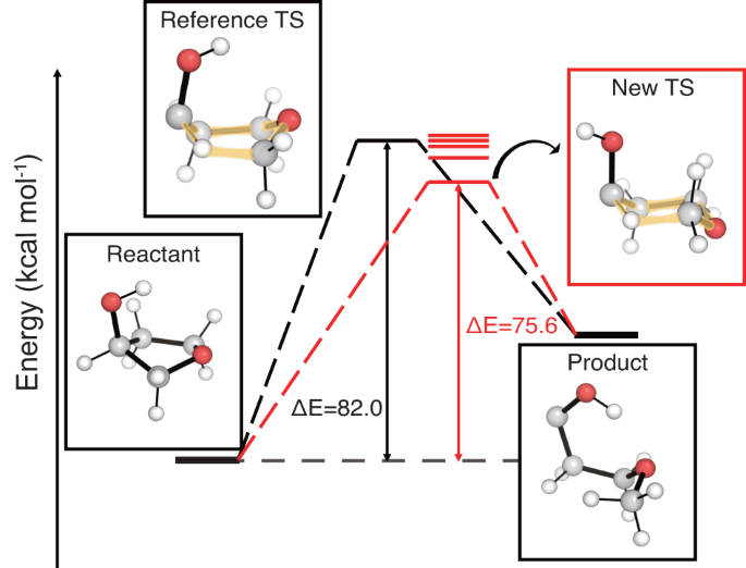
Figure 6 shows an example case where TSDiff found TS conformations with lower energies than that of the reference. Five different TS conformations were obtained by saddle point optimization, and their energy levels are indicated by the red lines. The lowest energy conformation in the red box has an energy 6.4 kcal mol⁻¹ lower than that of the reference, suggesting a more favorable reaction pathway. This substantial energy difference between the reference and the new TS conformations is due to the apparent geometric difference between them, where the hexagonal rings, highlighted in yellow, have the boat and chair conformations in the reference and the new TS, respectively. This emphasizes the importance of searching for different TS conformations to find a more favorable reaction pathway, and TSDiff can be used for this purpose. The results of the reaction conformational search utilizing TSDiff for more complex reactions can be found in the section Analysis on multiple reaction pathways explored by TSDiff.

**Fig. 6: Comparison of the barrier heights of the reference and those found by TSDiff.**

Analysis on failure cases

To further assess the coverage ability of TSDiff based on DFT calculations, we analyzed 199 reactions where the model failed to generate the correct TS within a single sampling. We performed up to four additional random samplings and validated the generated samples using the same process as in the previous section. This resulted in the identification of 89 correct TS geometries among 199. Of the remaining 110 reactions still not covered by TSDiff, we found that several samples were successfully optimized to their reference geometries but failed the IRC validation. We note that the IRC calculation of the reference TS may fail due to the lack of an IRC verification step during the data generation process^40,43.

Considering this point, we conducted IRC calculations on the reference TSs of the 110 reactions to confirm whether or not they are elementary step reactions. Among them, 95 reference TSs failed the IRC calculation, which highlights requirements of re-evaluating TSDiff’s performance on the remaining 1102 reactions after excluding them. Then, TSDiff achieved a success rate of 97.4%, with 8588 of the 8816 samples successfully optimized to the saddle point, as described in Table 3. The success rate of IRC validation for geometries generated by the single sampling was also recalculated to 90.6%, which was reported as 83.4% in the previous section. Finally, 98.6% of the refined test reactions were successfully covered by TSDiff within five rounds of sampling, which resulted in the correct TSs on 1087 reactions.

Table 3 Success rates of quantum chemical validations on geometries generated by TSDiff

Analysis on multiple reaction pathways explored by TSDiff

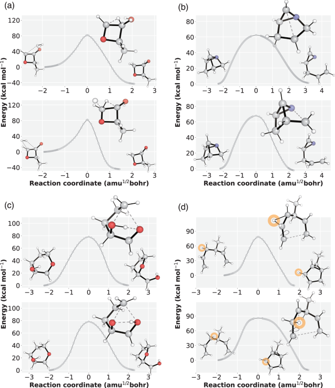
We present additional results for four reactions in which TSDiff discovered TS conformations with distinct reaction coordinates. For each reaction, two TS conformations were obtained by saddle point optimization of the generated TSs, resulting in D–MAE values between two conformations of 0.29 Å, 0.30 Å, 0.26 Å, and 0.15 Å for the four reactions, respectively. Subsequently, we obtained the energy profiles of the respective reaction pathways using IRC calculations. As a result, we identified two different reaction pathways for each reaction, despite both pathways sharing the same reaction graph. Figure 7 illustrates the IRC energy profiles of the reaction pathways along with the corresponding reactant, TS, and product geometries, clearly demonstrating the distinct reaction coordinates.

**Fig. 7: Intrinsic reaction coordinate (IRC) energy profile of four reactions.**

The reaction pathways depicted in Fig. 7a–c exhibit different bond breaking/formation sequences. For instance, Fig. 7a displays two reaction pathways with hydrogen molecules approaching from different directions in multimolecular reactants, highlighting the effectiveness of TSDiff in capturing TSs without considering alignments. In Fig. 7b, the top reaction involves cleavage of the C–C bond followed by the C–N bond, while the sequence is reversed in the bottom reaction. This difference is also evident in the bond lengths in the TS conformations shown in the figure. Similarly, in Fig. 7c, the top reaction involves cleavage of the C–O bond followed by the O–H bond, whereas the sequence is reversed in the bottom reaction. Furthermore, we observed the reaction with identical reactant and product, but involving different reactive atoms, as illustrated in Fig. 7d. In this reaction, a different hydrogen atom migrates to the neighboring carbon. For a clearer visualization, we have colored the migrating hydrogen atom in orange.

Source link