Data acquisition and preprocessing
This study explores how meta-level and statistical features of datasets affect ML performance. For this purpose, we considered 200 open-access tabular datasets from the Kaggle (147) and UCI Machine Learning Repository (53). Supplementary Table S1 details the source of these datasets. Each dataset addresses a binary classification problem, i.e., the targeted dependent variable can take one of the two possible values, either 0 or 1. Some sources have multiple datasets. For example, datasets D126–D174 are from the same Kaggle source, with the worldwide University ranking data from different ranking-producing organisations for various years. The same is true for datasets D175–D180, from the same UCI source for the Monk’s problem. Kaggle provides powerful tools and resources for the data science and AI community, including over 256,000 open-access datasets24. The UCI Machine Learning Repository collects over 650 open-access datasets for the ML community to investigate empirically25.
The datasets used in this study have attributes or variables of a wide range. These attributes can take an extensive range of values across datasets. Some appeared on a Likert scale, which captures textual opinions in a meaningful order26. For example, a response could be good, very good or excellent against a question of how you feel. We first changed such responses into a chronological numerical order. Second, the responses of some categorical attributes do not make an expressive numerical order. An example of such an attribute is gender, which can be male or female. A binary transformation of this attribute would lead to a bias, especially for the statistical mean or average feature. For a dataset with more male responses, if we consider 1 for males, that dataset’s mean or average feature will be larger and vice versa. Another example of such features is the marital status. For this reason, this study considers a target-based encoding to convert such categorical attributes to a quantitative score. The target-based encoding is an approach to replace a categorical variable using information from the dependent or target variable27. Third, the range for some attributes starts from a negative value. We shifted the range for those attributes so that its starting value is 0. If the range for an attribute is − 3 to 3, we move it from 0 to 6 by adding 3 to all instances. This study’s final preprocessing is to convert all attributes for each dataset into a range of 0 and 1 by following the min–max scaling approach28, which ensures their uniform value range across datasets. A dataset’s attribute (e.g., duration) can be 1–10 h. The value for another variable (e.g., age) of the same or different dataset may range between 18 and 120 years. We divide each instance of an attribute by the magnitude of the range of that attribute. For example, if the adult age range is 18–120 years of an attribute, we divide each instance by 102 (120–18). Such a normalisation also neutralises the impact of considering different units for the same attribute. Age could be in year or month, but the relative difference across instances will remain the same with this normalisation approach. The conversion of each attribute into a range of 0–1 ensures the quantification of each statistical feature is from the same value range across datasets.
Dataset features
This study considers three meta-level and four statistical features to investigate their influence on the performance of five classical supervised ML algorithms. We quantify these seven features and accuracy values against various ML algorithms for each dataset.
Meta-level features
For each dataset, this study considers three meta-level features. They are the number of attributes or variables used to classify the target variable, dataset size and the ratio between the number of yes (or positive) and no (negative) classes. A very high or low ratio value results in a class imbalance issue29. Hence, including this meta-level feature will help explore how the presence of class imbalance affects ML performance. The dataset size, or simply size, is the number of instances of that dataset. If a dataset consists of 100 cases with 60 positive and 40 negative samples, the ratio will be 1.25 (60 ÷ 40).
Statistical features
The four statistical features considered in this study for each dataset are mean or average, standard deviation, skewness and kurtosis.
Mean or average
For a set of \(N\) numbers \(({X}_{1},{X}_{2}\dots {X}_{N})\), the following formula can quantify the mean or average (\(\overline{X }\)) value.
$$\overline{X }=\frac{\sum_{i=1}^{N}{X}_{i}}{N}$$
Standard deviation
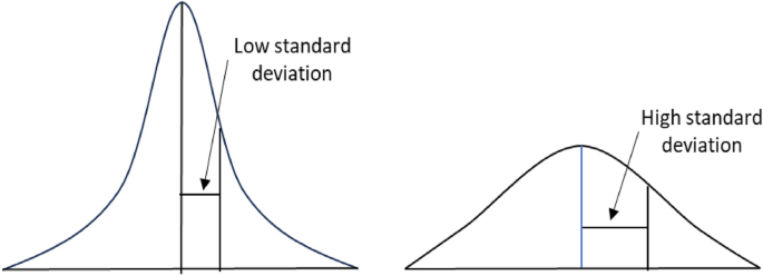
Standard deviation is a commonly used descriptive statistical measure that indicates how dispersed the data points are concerning the mean30. It summarises the difference of each data point from the mean value (Fig. 1). A low standard deviation of a given data demonstrates that its data points are clustered tightly around its mean value. Conversely, a high standard deviation indicates that data points are spread out over a broader range. For a dataset with size \(N ({X}_{1},{X}_{2}\dots {X}_{N})\) and mean \(\overline{X }\), the formula for the standard deviation (SD) is as follows.
$$SD=\sqrt{\frac{\sum_{i=1}^{N}{\left({X}_{i}-\overline{X }\right)}^{2}}{N-1}}$$
Skewness
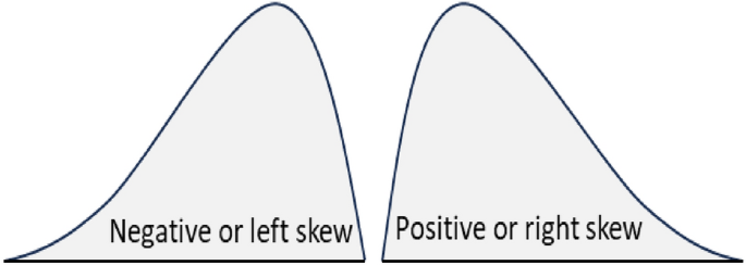
Skewness measures how far a particular distribution deviates from a symmetrical normal distribution30. The skewness value can be positive, zero or negative (Fig. 2). The left tail is longer for negatively skewed data. It is the right tail, which is longer for positively skewed data. Both tails are symmetrical for unskewed data. The following formula can measure the skewness (\({\widetilde{\mu }}_{3}\)) of a given data \(({X}_{1},{X}_{2}\dots {X}_{N})\).
$${\widetilde{\mu }}_{3}=\frac{\sum_{i=1}^{N}{({X}_{i}-\overline{X })}^{3}}{(N-1)\times {SD}^{3}}$$
where, \(\overline{X }\) and \(SD\) are the mean and standard deviation of the data, respectively. In the above formula, if the value of \({\widetilde{\mu }}_{3}\) is greater than 1, the distribution is right-skewed. It is left-skewed for \({\widetilde{\mu }}_{3}\) is less than -1. The tail region may be the source of outliers for skewed data, which could adversely affect the performance of any statistical models based on that skewed data. Models that assume the normal distribution of the underlying data tend to perform poorly with highly skewed (positive or negative) data30.
Kurtosis
For the probability distribution of a real-valued random variable, kurtosis quantifies the level of existing tailedness within that distribution30. It can identify whether the data are heavy-tailed or light-tailed relative to the normal distribution. Here is the formula to quantify the kurtosis (\({\beta }_{2}\)) of a dataset \(({X}_{1},{X}_{2}\dots {X}_{N})\) with mean and standard deviation of \(\overline{X }\) and \(SD\), respectively.
$${\beta }_{2}=\left\{\frac{N(N+1)}{(N-1)(N-2)(N-3)}\sum_{i=1}^{N}{\left(\frac{{X}_{i}-\overline{X}}{SD }\right)}^{4}\right\}-\frac{3{(N-1)}^{2}}{(N-2)(N-3)}$$
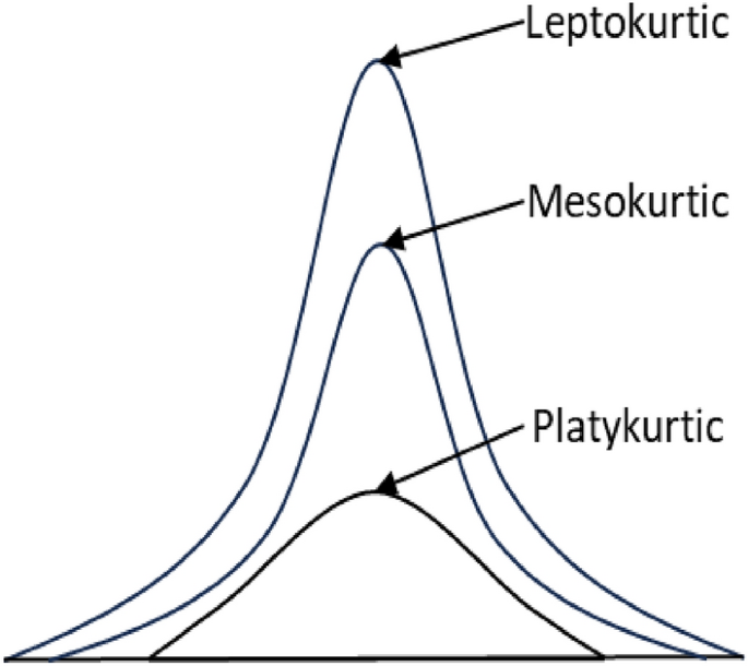
Based on the kurtosis value (\({\beta }_{2}\)), a distribution can be leptokurtic, mesokurtic and platykurtic (Fig. 3). A standard normal distribution has a kurtosis value of 3, known as mesokurtic. An increased kurtosis (> 3), known as leptokurtic, makes the peak higher than the normal distribution. A decreased kurtosis (< 3), known as platykurtic, corresponds to a broadening of the peak and thickening of the tails. Excess kurtosis indicates the presence of many outliers presented in the dataset, which could negatively impact the performance of any statistical models based on that dataset30.
Feature value quantification
The online open-access source for each dataset contains information on the number of attributes and instances (dataset size) with further details on the positive and negative splits. The third meta-level ratio feature has been calculated by dividing the number of positive cases by the number of negative instances. We followed the same approach to quantify each of the four statistical features for a given dataset. First, we calculated the underlying feature value for each dataset attribute. If the underlying feature is the skewness and the given dataset has six attributes, we then calculate the skewness of each attribute. After that, we aggregate these six skewness values by taking their average value. We also follow a weighted approach to aggregate them using each attribute’s principal component analysis (PCA) score as its weight. PCA is a popular dimensionality reduction technique that can assign scores to each feature based on their ability to explain the variance of the underlying dataset31.
Machine learning algorithms and experimental setup
This study considers five supervised ML algorithms to investigate how dataset features affect their performance. Two (Random forest and Decision tree) are tree-based, and the remaining three (Support vector machine, Logistic Regression and K-nearest neighbours) do not use any tree structure for the classification task.
Decision Trees (DT) are non-parametric methods partitioning datasets into subsets based on attribute values, though they can sometimes overfit3. Random Forest (RF) is an ensemble learning method that constructs multiple decision trees during training and outputs the mode of the classes for classification or the mean prediction for regression tasks, thereby reducing the overfitting risk associated with individual decision trees32. Support Vector Machine (SVM) classifies data by determining the best hyperplane that divides a dataset into classes2. Logistic Regression (LR) analyses datasets where independent variables determine a categorical outcome, commonly used for binary classification33. Lastly, the K-Nearest Neighbours (KNN) algorithm classifies an input based on the most common class among its nearest K examples in the training set. It offers versatility at the cost of computational intensity34.
This study used the Scikit-learn library35 to implement the five ML algorithms with the 200 open-access tabular datasets considered in this study. Each dataset underwent an 80:20 split for the training and test data separation. We followed a five-fold cross-validation for training model development. For other experimental setups, this study used the default settings of the Scikit-learn library. Moreover, this study considered accuracy as the performance measure for ML algorithms. It represents the percentage of correct classifications made by the underlying ML model. In addition to the basic implementation using the Scikit-learn library, this study implemented all ML algorithms through hyperparameter tuning of different relevant parameters. Hyperparameter tuning is selecting a set of optimal parameters for the ML algorithm to boost its model performance36. We used the GridSearchCV function from Scikit-learn to tune different hyperparameters for different ML algorithms, such as the kernel type and C value for SVM and the k value in KNN.
After quantifying three meta-level and four statistical features and the ML accuracy for each of the 200 tabular datasets, this study applied multiple linear regression to explore their impact on ML performance. We used IBM SPSS Statistics software version 28.0.0.037 for multiple linear regression modelling.


