This blog post is an overview of some recent work, lead by my co-author Adam
Yang (Yang et al., 2024), in which we tackle the issues of
over-confidence in large language models and poor calibration, particularly
when fine-tuned on small datasets or small collections of human feedback.
Taking a Bayesian approach, our method estimates the per-logit uncertainty over
the next predicted token. This is particularly useful, for instance, for
multiple choice question answering, classification tasks or reward modelling.
We can also use our method to calculate the model evidence in order to tune
model hyperparameters.
Crucially, our method is applied as a post-hoc modification to a fine-tuned
network
0: that is; can be applied following a similar workflow to existing
post-training quantization methods such as AWQ
(Lin et al., 2023)
0[0]
, meaning that the standard,
highly-optimised pre-training and fine-tuning pipelines can remain exactly the
same, and the method can be applied to previously LoRA-finetuned
models
1: or even fully fine-tuned models, although the computational cost of
our method will be higher in this case
1[1]
.
TL;DR:
- When fine-tuning an LLM, how do you know if your model has learned
to perform the task well? - Normally, the LLM only predicts the categorical parameters (logits)
- Our method additionally provides the variance (uncertainty) in these logit
predictions (a Bayesian predictive distribution over the logits) - the more fine-tuning data we see, the narrower the distribution, and the more
certain our model is - Most useful for single-token prediction tasks: reward modelling or
multiple-choice question answering - We can also calculate the model evidence to tune model hyperparameters
- Try it out with our library
(pip install bayesian-lora)
One notable property of large langauge models is that they have rather
good calibration curves coming out of pre-training, and that the quality of the
calibration swiftly deteriorates after fine-tuning
2: RLHF, or otherwise
2[2]
.
For instance, the GPT-4 technical report
(OpenAI, 2023)
3: to be pedantic, this chart was
produced in the full weight finetuning setting and not with LoRA adapters, yet
the point still holds
3[3]
illustrated this nicely with the following figure:
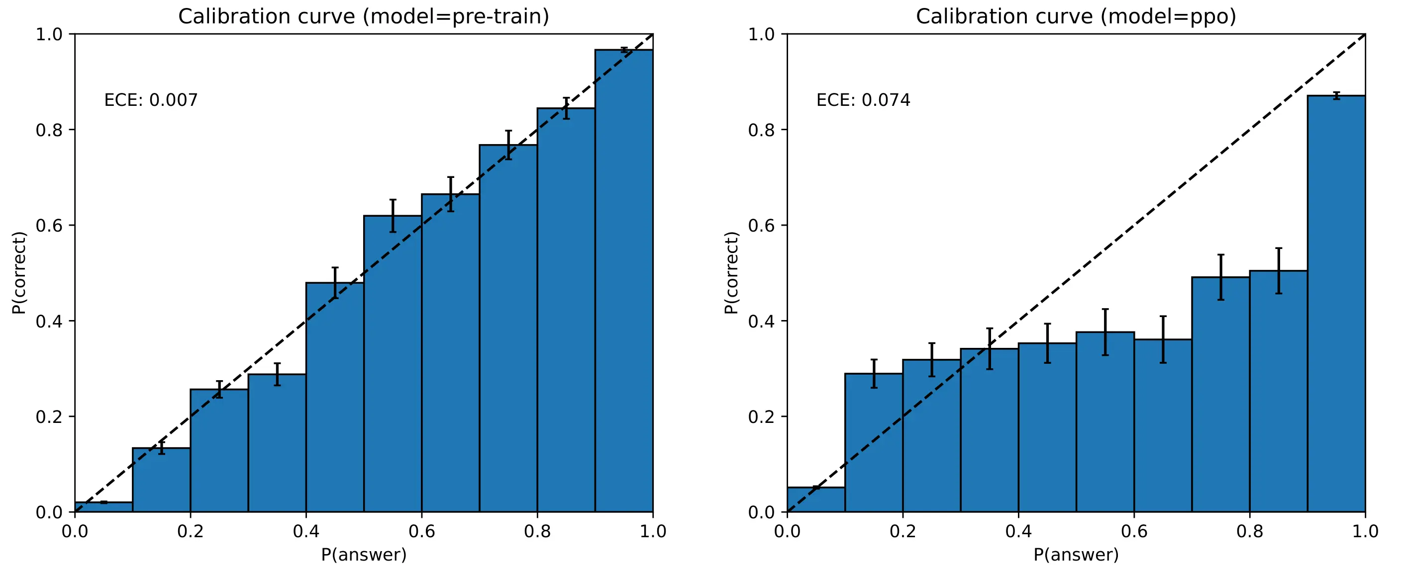
GPT-4 calibration curves for both the base pre-trained model and a PPO-finetuned model, evaluated on MMLU.
For those unfamiliar with calibration curves, we want the model to be confident
if its predictions are correct, and—perhaps most importantly—‘un-confident’
when its predictions are incorrect.
For instance, in a multiple choice task
4: we can predict classes in an
autoregressive language model with a single next-token prediction by merely
selecting the tokens corresponding to the class label (e.g. “ A”, “ B”, “ C” and so on) while disregarding all other tokens.
4[4]
if a model predicts some class “A” with 70% confidence, and it is a well
calibrated model, then in reality class “A” should be the correct answer about
70% of the time in the dataset. For a poorly calibrated model, we
would expect class “A” to be correct \(p \ne 70\)% of the time. Ideally, our
models would have \(\P(\mathrm{answer}) = \P(\mathrm{correct})\) everywhere.
Our method provides a Bayesian predictive distribution over the model’s
logits.
Where a model might have previously placed 90% of its confidence behind a
single logit, our method provides us with a predictive distribution over this
logit’s value
5: at risk of being ambiguous, our method isn’t constrained to
single-logit predictions; we can predict the distribution over a single logit,
a subset of logits, or all the logits
5[5]
; allowing us to examine the variance
hence the level of uncertainty
6: that is, the uncertainty due to lack of data
/ test distribution shift; influenced by the chosen prior
6[6]
in this prediction
which appears confident if we only look at the point estimates of the logits.
Why Fine-Tuning?
There has been some previous interest in bringing Bayesian inference to
LLMs, however most of this work has focused on the pre-training setting
(Xue et al., 2021; Cinquin et al., 2021; Chen et al., 2022).
As some of these works themselves conclude, there is little to be
gained from a Bayesian treatment of the pre-training setting; where the
abundance of data—the trillions of
tokens—drives uncertainty low for in-distribution test points, the models are
surprisingly well calibrated (Kadavath et al., 2022) and the
additional cost of the Bayesian machinery becomes exorbitant.
In contrast, the advantages of Bayes become more apparent in the fine-tuning
setting, where the smaller datasets tend to yield poor calibration
(OpenAI, 2023). Further, the popularity of LoRA
adapters (Hu et al., 2022) for model fine-tuning provides a
significant reduction in the number of parameters we need to consider, which
goes some way towards making the usually expensive Bayesian methods applicable
to language models. Our method—described below—is based on a Laplace
approximation, with a Kronecker-factored approximation to the Fisher
(MacKay, 1992; Daxberger et al., 2022). In addition, the alternating
wide-then-narrow shapes of LoRA adapters’ layers affords our method a
particularly efficient low-rank approximation to the Kronecker-factored
approximate curvature
(Eschenhagen et al., 2023), further reducing
the memory cost of (approximate) Bayesian inference in the LLM .
Hence, our method can be applied to fine-tuned models, to estimate
the uncertainty in each token’s prediction. While we focus on LoRA
fine-tuning, this isn’t necessary beyond reducing the memory cost, and our
method can be applied to full fine-tuning too.
What follows is a short overview of our method, which we call Laplace
LoRA—for the full details, refer to the paper.
Parameter-Efficient Fine-Tuning
As set out in the introduction, we consider parameter-efficient fine-tuning of
LLMs using low-rank adapters (Hu et al., 2022). For any
given weight matrix \(\rmW \in \R^{m \times n}\), mapping \(n\)-dimensional inputs
to \(m\)-dimensional outputs, a LoRA adapter is just a low-rank weight
perturbation \(\Delta\rmW = \rmB\rmA\), parametrised by \(\rmB \in \R^{m \times r}\) and \(\rmA \in \R^{r \times n}\), which, when added to \(\rmW\), alters the behaviour of that
layer.
Letting \(\rva \in \R^{n}\) be the input activation to the layer, and \(\rvs \in \R^{m}\) the
pre-activations, the forward pass becomes:
\[\begin{equation}
\label{eq:lora}
\rvs = (\rmW + \Delta\rmW)\rva = (\rmW + \rmB\rmA)\rva = \rmW\rva + \rmB\rmA\rva.
\end{equation}
\]
We usually set rank \(r\) of this adapter to some \(r \ll \min(m, n)\) to get a
low-rank adapter. Visually,

In transformers, typically \(m = n \approx 4096\), and we often select fairly low
ranks such as \(r \approx 8\). During normal training or fine-tuning, the number
of parameters in this linear layer is \(mn\) (e.g. 16.7 million) while in
LoRA fine-tuning, we freeze \(\rmW\) and only have \(rn + rm\) (e.g. 65
thousand) trainable parameters as a result—a significant reduction which
makes a Bayesian treatment of these parameters feasible.
Laplace Approximations
So far, everything has resembled standard fine-tuning.
We are now interested in finding a distribution over the fine-tuned weights,
such that we can calculate the model evidence or the predictive distributions.
For this, we use a Laplace approximation, which represents the weight posterior
as a Gaussian, centred at the maximum a-posteriori weights, and with covariance
equal to the Fisher information matrix.
Posterior Approximation
Let \(\vtheta\) denote all the trainable
7: that is, distinct
from all the weights in the LLM, which may exclude frozen and quantized
pre-trained model weights
7[7]
weights of our network.
We’ll also use \(\rmX \in \gV^{B \times N}\)
to denote the inputs to the LLM, with \(\gV\) the vocabulary
set
8: or set of possible tokens
8[8]
, \(B\) the batch size, and \(N\) the (maximum;
i.e. left-padded) sequence length. The targets are \(\rvy\in\gY^{B}\), where
\(\gY\) could differ
from \(\gV\) (e.g. multiple choice question answering, sentiment classification)
or it could be the same as \(\gV\) (e.g. next token prediction, autoregressive
decoding).
For models trained with a cross-entropy loss, the likelihood \(\P(\rvy \vert \rmX, \vtheta)\) is just a Categorical distribution, with logits given by the
network prediction \(f_{\vtheta}(\rmX)\).
For the prior distribution over the fine-tuning weights, we simply use an
isotropic Gaussian prior with precision \(\lambda\):
\[\begin{equation}
\label{eq:lora_prior}
\P(\vtheta) = \gN(\mathbf{0}, \lambda^{-1}\rmI).
\end{equation}
\]
Note that a normal training run (i.e. minimising a cross entropy loss with
weight decay) is equivalent to maximising a log joint, \(\log \P(\rvy, \rmX, \vtheta)\) with this likelihood and prior.
That is, it is equivalent to maximising the following:
\[\begin{align}
\log\P(\gD, \vtheta) &= \log \P(\rvy \vert \rmX, \vtheta) + \log \P(\vtheta) \label{eq:log_joint} \\
&= \log \P(\rvy \vert \rmX, \vtheta) + \log \gN(\vtheta; \mathbf{0}, \lambda\rmI) \\
&= \log \P(\rvy \vert \rmX, \vtheta) + \frac{\lambda}{2}\Vert \vtheta \Vert_{2}^{2} + \mathrm{const}. \\
&\doteq \gL(\rvy, \rmX; \vtheta).
\end{align}
\]
We can see that the effect of the prior in Equation \(\ref{eq:lora_prior}\) is
the same as regularising the L2 norm of the weights; in other words, applying
weight decay with a strength of \(\lambda / 2\).
Hence, we can re-use the weights from any previous training run with sensible
weight decay (e.g. optimised with AdamW, where the default weight decay is
\(0.01\)).
Since we’re after the posterior distribution over the weights after fine-tuning, we need
to calculate:
\[\label{eq:llm_weight_posterior}
\begin{equation}
\P(\vtheta \vert \rmX, \rvy) = \frac{\P(\rvy \vert \rmX, \vtheta) \P(\vtheta)}{p(\rmX, \rvy)}.
\end{equation}
\]
The marginal likelihood in the denominator is usually intractable, so we turn
to one of the many approximations in the Bayesian’s toolbox; in this case the
Laplace approximation (MacKay, 1992; Daxberger et al., 2022).
We start with the regularised training solution
(i.e. maximising \(\gL(\rvy, \rmX; \vtheta)\)),
which we will refer to as the maximum a-posteriori solution
(\(\vtheta_{\mathrm{MAP}}\)) henceforth:
\[\begin{align}
\gL(\rvy, \rmX; \vtheta) &= \log \P(\rvy \vert \rmX, \vtheta) + \log \P(\vtheta) = \log \P(\vtheta \vert \rmX, \rvy) + \mathrm{const}. \\
\vtheta_{\mathrm{MAP}} &= \argmax_{\vtheta}\gL(\rvy, \rmX; \vtheta).
\end{align}
\]
Now, taking a second-order Taylor expansion of the log-joint around
\(\vtheta_{\mathrm{MAP}}\), we get
\[\begin{equation}
\label{eq:log_joint_taylor}
\gL(\rvy, \rmX; \vtheta) \approx \gL(\rvy, \rmX; \vtheta_{\mathrm{MAP}}) – \frac{1}{2}(\vtheta – \vtheta_{\mathrm{MAP}})^{\top}\big(-\nabla_{\vtheta}^{2}\gL(\rvy, \rmX; \vtheta)\vert_{\vtheta_{\mathrm{MAP}}}\big)(\vtheta – \vtheta_{\mathrm{MAP}}).
\end{equation}
\]
Notice that the first-order term in Equation \(\ref{eq:log_joint_taylor}\)
disappears, on account of the gradient of the log-joint being \(0\) at the
MAP parameter location
9: That is, we’d expect the gradient of the MAP
objective, evaluated at the MAP parameter location, to be (approximately) zero
after training.
9[9]
, and we have written the second-order term in negated form by
negating the Hessian inside the brackets
10: This is just
to make matching terms more explicit later.
10[10]
.
Now, matching terms with the quadratic forms in Equations
\(\ref{eq:log_joint_taylor}\) and a log Gaussian density, we arrive at the
Laplace approximation of the unnormalised posterior \(\P(\vtheta \vert \rmX, \rvy)\) as a Gaussian centred at \(\vtheta_{\mathrm{MAP}}\) with precision
\(\mLambda_{\mathrm{post}}\):
\[\begin{align}
\P(\vtheta \vert \rmX, \rvy) &\approx \gN(\vtheta; \vtheta_{\mathrm{MAP}}, \mSigma_{\mathrm{post}}) \\
\mSigma_{\mathrm{post}} &= \mLambda_{\mathrm{post}}^{-1} \\
\mLambda_{\mathrm{post}} &= -\nabla_{\vtheta}^{2}\gL(\rvy, \rmX; \vtheta)\vert_{\vtheta_{\mathrm{MAP}}} \\
&= -\nabla^{2}_{\vtheta}\log \P(\rvy \vert \rmX; \vtheta)\vert_{\vtheta_{\mathrm{MAP}}} – \nabla^{2}_{\vtheta}\log \gN(\vtheta; \mathbf{0}, \lambda^{-1}\rmI)\vert_{\vtheta_{\mathrm{MAP}}} \\
&= -\nabla^{2}_{\vtheta}\log \P(\rvy \vert \rmX; \vtheta)\vert_{\vtheta_{\mathrm{MAP}}} + \lambda\rmI \label{eq:sigma_post_terms}.
\end{align}
\]
There are however two issues with \(\mLambda_{\mathrm{post}}\). The first is that
we need it to be positive definite; looking at the first term in Equation
\(\ref{eq:sigma_post_terms}\), we see that this is the case if the likelihood is
convex at \(\vtheta_{\mathrm{MAP}}\), and of course the outputs \(\rvy\) are within
the support of the likelihood
11: i.e. \(\P(\rvy \vert \rmX; \vtheta) > 0\),
where the inequality is strict
11[11]
. However with complicated neural network
likelihoods, this local convexity condition is not guaranteed to hold. The
second issue with \(\mLambda_{\mathrm{post}}\) is that it is a very large \(P \times P\) matrix, where \(P\) is the number of elements in \(\vtheta\), making it
impractical to work with directly.
Fisher Information
To resolve the first of these issues, we instead use the Fisher information
matrix instead of the Hessian directly. The Fisher is defined
12: do see my
previous article on second order methods to gain some
intuition about this quantity.
12[12]
as:
\[\begin{equation}
\label{eq:fim}
\rmF(\vtheta) \doteq \E_{\substack{\hat{\rvx} \sim \gD \\ \hat{\ervy} \sim \P(\rvy \vert f_{\vtheta}(\hat{\rvx}))}}\left[\nabla_{\vtheta}\P(\hat{\ervy} \vert f_{\vtheta}(\hat{\rvx}))\big(\nabla_{\vtheta}\P(\hat{\ervy} \vert f_{\vtheta}(\hat{\rvx}))\big)^{\top}\right],
\end{equation}
\]
where we use \(\hat{\ervy} \sim \P(\rvy \vert f_{\vtheta}(\hat{\rvx}))\) to
denote samples drawn from the model’s output distribution. This is now a
positive semi-definite matrix, which resolves the first of our two issues.
Kronecker-Factored Approximate Curvature
To reduce the memory requirements, we use a low-rank Kronecker-factored
approximation to the curvature. This involves three approximations:
1. We first treat the Fisher information as a block-diagonal matrix (i.e. treating each of the network’s layers \(L1, L2, \ldots\) independentally)

2. Following the standard K-FAC procedure
(Martens et al., 2015), we further factorise each of these
blocks \(\rmF_{\ell\ell}\) as a Kronecker product of two smaller matrices,
\(\rmA_{\ell-1}\) and \(\rmS_{\ell}\). These correspond to the expected outer
product of layer \(\ell\)’s input activations \(\rva_{\ell-1}\) and output
gradients \(\gD\rvs_{\ell} \doteq \nabla_{\rvs_{\ell}}\log \P(\rvy \vert \rmX; \vtheta)\), respectively, where \(\rvs_{\ell}\) is the pre-activation output of
layer \(\ell\). That is,
\[\begin{equation}
\label{eq:kfac}
\rmF_{\ell\ell} \approx \underbrace{\E\left[\rva_{\ell-1}\rva_{\ell-1}^{\top}\right]}_{\rmA_{\ell-1}} \otimes \underbrace{\E\left[\gD\rvs_{\ell}\gD\rvs_{\ell}^{\top}\right]}_{\rmS_{\ell}},
\end{equation}
\]
where the expectations are as in Equation \(\ref{eq:fim}\). Note that this second
approximation comes not from the Kronecker factorisation, but the independent
expectations.
3. Despite \(\rmA_{\ell-1}\) and \(\rmS_{\ell}\) being smaller than
\(\rmF_{\ell\ell}\), the first factor scales as the square of the layer’s input
width, while the second factor scales as the square of the layer’s output
width.
Since we are working with LoRA adapters, layers \(\ell\) alternate between
wide-input-narrow-output and vice versa; hence one of the two Kronecker factors
will be very large (e.g. \(4096 \times 4096\)), while the other will be very
small (e.g. \(8 \times 8\)).
To this end, we use an incremental
13: that is, to avoid having to materialise
the full matrix and run a big SVD, we incrementally compute the SVD as we
iterate over batches
13[13]
SVD to estimate the larger of these factors as a
product of two new low-rank factors. For example if \(\rmA_{\ell-1} \in \R^{d \times d}\) is the larger factor, we approximate it as \(\rmA_{\ell-1} \approx \rmB\rmB^{\top}\) for some \(\rmB^{d\times n_{\mathrm{kfac}}}\); thus saving
memory.
Linearized Prediction
All the above was to get a tractable way of obtaining the paramters of our
Gaussian approximate posterior. Recall, that the posterior is a Gaussian
\(\P(\vtheta \vert \rmX, \rvy) \approx \gN(\vtheta; \vtheta_{\mathrm{MAP}}, \mSigma_{\mathrm{post}})\), centred at the
MAP parameter locations (e.g. from a previous training run), with a
block-diagonal covariance matrix given by the inverse of our low-rank
K-FAC scheme (plus the diagonal prior term).
We can now use this posterior to make predictions. The Laplace approximation
has strong connections to linearising the network
(Antorán et al., 2022), and it is often found that
predicting from a linearised model is more effective than doing the intuitive
thing of sampling a set of weights from the posterior and using those to
predict using the full network. That is, for some test input \(\rvx_{\star}\),
the linearised network is
\[\begin{equation}
\label{eq:linearised_net}
f_{\vtheta}(\rvx_{\star}) \approx f_{\vtheta_{\mathrm{MAP}}}(\rvx_{\star}) +
\nabla_{\vtheta}f_{\vtheta}(\rvx_{\star})\vert^{\top}_{\vtheta_{\mathrm{MAP}}}(\vtheta
– \vtheta_{\mathrm{MAP}}).
\end{equation}
\]
This is now just a linear transformation of the Gaussian-distributed weights,
hence we can easily integrate these out
14: see my previous
article on Gaussians for more on this
14[14]
to
get a Gaussian predictive distribution on the output logits:
\[\begin{equation}
\label{eq:posterior_predictive}
f_{\vtheta}(\rvx_{\star}) \sim \gN\big(\rvy; f_{\vtheta_{\mathrm{MAP}}}(\rvx_{\star}), \mLambda\big),
\end{equation}
\]
for
\[\begin{equation}
\label{eq:post_pred_cov}
\mLambda = \big(\nabla_{\vtheta}f_{\vtheta}(\rvx_{\star})\vert^{\top}_{\vtheta_{\mathrm{MAP}}}\big)\mSigma_{\mathrm{post}}\big(\nabla_{\vtheta}f_{\vtheta}(\rvx_{\star})\vert_{\vtheta_{\mathrm{MAP}}}\big).
\end{equation}
\]
Decomposing the above using a Cholesky decomposition, \(\mLambda = \rmL\rmL^{\top}\), we can draw posterior samples using reparametrised sampling:
\[\begin{equation}
\label{eq:reparam_sampling}
\hat{\rvy} = f_{\vtheta}(\rvx_{\star}) = f_{\vtheta_{\mathrm{MAP}}}(\rvx_{\star}) + \rmL\vxi, \hskip{2em}\vxi \sim \gN(\mathbf{0}, \rmI).
\end{equation}
\]
Marginal Likelihood
Finally, we can also use the marginal likelihood (or model evidence), which
we have in closed form owing to our Laplace approximation, to optimise
hyperparameters such as our selected prior precision. The marginal likelihood
can be approximated in closed form as
\[\begin{align*}
\P(\rvy \vert \rmX) &= \int \P(\rvy \vert \rmX; \vtheta)\P(\vtheta) d\vtheta \\
&\approx \exp\big(\gL(\rvy, \rmX; \vtheta_{\mathrm{MAP}})\big)(2\pi)^{D/2}\det(\mSigma_{\mathrm{post}})^{1/2}.
\end{align*}
\]
This quantity can be used as an objective to tune the value of \(\lambda\) for
instance.
Do look at the accompanying
repository and the
documentation for
code examples.


