Anaerobic system and data collection

The data for the present study was obtained from a two-stage laboratory scale anaerobic treatment reactor installed at Jaipur, India³². Figure 1 shows the reactor used in the present study and its experimental setup. The two-stage reactor consisted of two semi-cylindrical chambers, created by dividing a single cylindrical unit into two parts as illustrated in Fig. 1. The first chamber worked as a modified septic tank and the second one as an anaerobic filter to perform post-treatment of the modified septic tank effluent. The second chamber was randomly packed with media and fed with the effluent of the first chamber, which entered it from the bottom. The media (baked clay of 20 mm size) was kept on a semi-circular perforated plastic plate, placed at a height of 60 mm from the bottom of the tank. The total effective volume of the two-stage system was 24 L having unit dimensions of 450 mm of height and 300 mm of diameter.

Line diagram of two-stage anaerobic treatment reactor.

All experiments were carried out in the two-stage anaerobic treatment reactor under different operating conditions. The concentrations of all parameters of actual domestic wastewater injected into the system varied greatly. The system was started without vaccination and was operated for a long time. Monitoring during the study period was carried out at temperature range of 17–45 °C. The efficiency of anaerobic treatment was examined at different hydraulic and organic loading rates.

The anaerobic two-stage treatment unit was continuously fed with water at a constant flow rate of 24 L/day, equal to 24 h hydraulic retention time (HRT), until the system reached steady state. All wastewater resulting from domestic activities flowed directly to the treatment facilities without changing its properties. It was then fed with domestic wastewater that was collected on a daily basis. For a week, the reactor was maintained in anaerobic conditions. After that, it was fed with household wastewater that collected on daily basis.

Temperature was found to have an impact on the anaerobic biodegradation of organic matter over the research period. Wastewater temperature was found to change during the day by 11–49 °C. Figure 2 shows how temperature changes affect the effectiveness of COD removal. When the system was first started in the winter, it was noted that when the temperature rose over time, the system’s total COD removal effectiveness improved. When sewage reached its maximum temperature of 45 °C, 92.5% COD removal effectiveness was recorded.

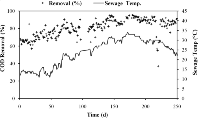
Changes in COD elimination effectiveness with temperature.

The input parameters were measured from wastewater drawn from the points of influent, and effluent parameters from the outlet of the secondary chamber. Following influent and effluent parameters were analyzed by standard procedure (APHA):

1. a.

   Total alkalinity (T. Alkalinity (mg/L)),

2. b.

   Influent chemical oxygen demand (inf CODT (mg/L))

3. c.

   Influent soluble chemical oxygen demand (inf. SCOD (mg/L)),

4. d.

   Total suspended solids (TSS (mg/L)),

5. e.

   Influent Kjeldhal nitrogen (inf. TKN in mg/L)

6. f.

   NH₃⁻N (ammoniacal nitrogen (mg/L)) and

7. g.

   NO₃⁻N (nitrate nitrogen (mg/L).

ADM1 performance

Modified ADM1 was developed according to two-stage anaerobic treatment reactor to predict effluent COD from modified ADM1. To accomplish this goal, the modelling and simulation of anaerobic digestion of household wastewater was conducted using elemental analysis and ADM1³³.

Table 1 summarizes the reactors’ liquid phases as well as the key ADM Model parameters that were employed in this investigation.

In accordance with the experimental setup, data has been collected for 365 days. The input parameters were measured from wastewater are drawn from the points of influent and effluent parameters from the outlet of the secondary chamber. Following influent and effluent parameters were analyzed by standard procedure (APHA):

Few assumptions made while developing the model are explained below.

• The concentration of input oxygen was assumed to be zero.

• Particulate substrate and inert particulate material were the only parameters considered to be present in primary wastewater.

• The influent included a reasonable amount of nitrogen.

The analysis’s findings were converted to the appropriate units. The Matlab program developed for the elemental analysis approach that used the data as input. The stoichiometric coefficients for the empirical formula and the fractions of proteins, fats, carbohydrates, and volatile fatty acids (VFA) were the output results. The typical ADM1 model required a COD-based substrate concentration specification, but the equations for determining the substrate composition were expressed as C-molar fractions of the substrates. Based on converting fractions to COD, equivalent concentration was determined. For carbohydrates³⁴, it is as follows:

where the number 4 represented the number of electrons that were accepted per mole Oxygen and MWO₂ was the molecular weight of oxygen. The findings of the simulation were compared to the COD measurements obtained from the two-stage reactor following the treatment of domestic wastewater.

Based on the inlet concentration in raw domestic wastewater, a comparison of the measured and simulated effluent SCOD was also carried out (Fig. 3). The findings showed that there was a minor variation between the simulated and measured effluent data because the samples contained inorganic suspended particles also. The output from the ASM2ADM interface is displayed against the experimental SCOD as shown in Fig. 3.

SCOD value variation from experiments with the ASM2ADM interface.

Figure 3 illustrates the comparison between the measured SCOD and predicted SCOD values. The figure shows that the predicted values of SCOD closely matched with the measured values. To validate the results obtained from ADM1, machine learning techniques were used.

Machine learning techniques

Four machine learning techniques, namely Linear regression, Decision Tree, Random-Forest, and Artificial Neural Networks (ANN) were used in the present study. The collected data for different input variables were normalized in accordance with Interquartile ranges. To enhance the quality of data, statistical techniques were applied leading to better classification through normalization.

Data pre-processing

Data pre-processing is the primary step that is performed for any data-driven analysis. For our purpose, the data normalization method was used. As the name implies, data normalisation is the process of improving the quality of data to improve classification. Redundancy and inconsistency must be eliminated by data normalisation. Null values were examined first for garbage in this study. These entries were removed from the database. By employing the equalisation histogram, the pre-processed database was normalised. Feature extraction and machine learning step were now possible. The data was then further refined for feature extraction and machine learning phase.

Feature selection

Initially, a correlation matrix is formulated to relate the input variables with each other. In this phase correlation matrix and mutual information gain are applied to filter out the most important features and remove duplicate features, if any. Correlation matrix denotes the correlation between different variables (input variables) for predicting target variable. High correlation denotes that the two variables affect the target variable similarly; therefore, one can be dropped from the analysis. Mutual Information Gain represents the significance or influence of input variables for predicting target variable. Input variables with high mutual information gain and less correlation were selected, and the others were discarded, thereby reducing computational overhead without affecting the performance. The steps involved in the process are listed below.

• Constant value features checking (Check 0 variance between the feature’s columns value).

• Check if there are any feature columns whose values are 99% same.

• Check feature importance or decide features’ ranking using correlation checking.

• Check features’ importance using mutual information gain.

Figure 4 represents the correlation matrix of the features, and Fig. 5 represents the importance of each feature based on mutual information gain.

Correlation matrix of seven input variables.

Mutual information gain value of the seven input variables.

It can be inferred that influent TKN and influent COD_T are 95% correlated. One can be assessed if the other parameter is known. Hence, for the study, influent TKN was omitted, and influent COD_T was considered. Table 2 gives the descriptive statistics of the final six input variables and Table 3 shows the descriptive statistics of the effluent soluble COD after normalization and Feature extraction.

Predicting SCOD with machine learning

In Machine Learning, the trained models are validated by checking the effluent SCOD prediction on testing dataset and comparing the similarity between actual and predicted values of effluent SCOD. In the present research, effluent SCOD was the target variable, which was predicted based on 6 most important features (inf SCOD, inf CODT, TAlkalinity, TSS, inf NH₃-N, and inf NO₃-N) as selected in section “Feature selection“.

A series of specialized algorithms is created in machine learning process to recognize the pattern of data, classification, and prediction. The machine learning techniques are quite effective in finding trends in databases that are highly unstructured. In the present study, three algorithms of machine learning, namely ANN, random forest, and decision tree, were used for classification. Traditionally for binary classification, linear regression is utilized as a statistical approach which has become a popular machine learning tool.

In statistics, linear regression refers to a linear method that models the relationship between a scalar response and one or more independent variables. In linear regression, relationships are modeled with linear predictive functions, and the variable parameters of these functions are estimated from the data. In most cases, it is assumed that the conditional mean of the response to the values of the independent variables is an affine map of these values. Other statistical measurements, such as conditional median, were also used. The primary objective of linear regression is conditional probability distribution of the variables. Multivariate analysis, on the other hand, focuses on joint probability distribution.

A decision tree is a sequence model that logically integrates a series of simple tests. In each test, a defined numerical attribute is compared to a set of possible values. As Logical rules used by a decision tree can be easily understood, these symbolic classifiers are more coherent and intelligible than black box models, such as neural networks. Data analysts and decision makers usually prefer an easy-to-understand model. When a data point enters a partitioned area, the decision tree classifies it as the most common class in the area.

Random Forests are sometimes described as Random Decision Forests. It is an ensemble learning technique for classification and regression that uses multiple decision trees and training phases. The mode or mean anticipated value of the results from each decision tree is the output class. To create a single decision tree, a random cell from the given data was chosen. As the association between the individual trees is lessened by randomly choosing the features, random forests have a very high predictive power.

The ANN is an effective computing tool which ismodelled after the structure and processing capabilities of biological neurons, such as those found in human brain. Similar to human brain, an artificial neural network is made up of simple processing units (called nodes) that interact with one another and process local data. The input signal is received by each node in the network, which then processes it and delivers an output signal to the other nodes. Each node must be connected to at least one other node, and the weight coefficient, a real integer, measures the significance of each connection (synapse). The architecture of the Neural Network topology is demonstrated in Fig. 6.

Architecture of neural network.

The input variables in the study and the data collected from influent wastewater are represented by the input neurons. The output and target effluent SCOD is represented by output neuron. With 307 input data points, a 6–1–1 neural network structure was created to train the effluent COD prediction model. The network was trained using a feed-forwardback propagation model, in which a generalised delta rule was used to modify the link weights and biases between the neurons by propagating the mistake at the output neurons backward to the hidden layer neurons and subsequently to the input layer neurons. The study used a tangent sigmoid activation function in the output-layer and a logging transfer function at the hidden layer. The Levenberge-Marquardt backpropagation technique built into the Matlab® Neural Networks Toolbox was used for the training.